1.Introduction
Version 2024
This documentation specifies the format of datasets for the MonolixSuite starting in 2018. It details:
- General structure: structure of a dataset for population modeling
- Format rules: rules to format your experimental data, using the available column types
- Examples: examples of real datasets with typical features (continuous data, discrete data, time-to-event data, censored data, data with several types of measurements, …)
- Nonmem differences: key differences with the Nonmem format
©Lixoft
Dataset for population modeling
The considered datasets are dedicated to population modeling. The population approach describes phenomena observed in each of a set of individuals and the variability between individuals. The data is thus individual data, and is often longitudinal (over time). For each subject, the dataset contains measurements, dose regimen, covariates etc … i.e. all collected information.
General format
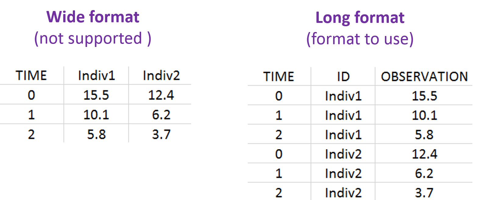
The data must be in long format, i.e each row is one time point per subject. For each row, the individuals ID, observations, dose amount, covariates, etc are recorded in different columns. The column names in the dataset header can be set to anything, but the columns must be tagged using the available column types when defining the data in the applications of the MonolixSuite, such that the application knows how to interpret the data. The column types are very similar and compatible with the structure used by the Nonmem software.
File types: The file should be in text format with a file of .txt or .csv or .tsv. and the data must be separated by tab “\t”, comma “,”, semicolon “;” or a space ” “. A header line is required specifying the column names. Additionally, starting with version 2024, Excel files with extensions .xls or .xlsx and SAS files with extensions .sas2bdat, and .xpt are supported.
2.Population modeling data set description
Data set structure
The data set structure contains for each subject measurements, dose regimen, covariates etc … i.e. all collected information. The data must be in the long format, i.e each line corresponds to one individual and one time point. Different type of information (dose, observation, covariate, etc) are recorded in different columns, which must be tagged with a column type (see below). The column types are very similar and compatible with the structure used by the Nonmem software (the differences are listed here).
Description of line-types
Depending on the information it contains, each line will be considered as (with exception of the header line):
- dose-line: line that contains information about the dose’s regimen (and possibly also about covariates and regression variables)
- response-line: line that contains an observation (and possibly also about covariates and regression variables)
- both dose and response-line: line that contains information about both the dose regimen and an observation (and possibly also about covariates and regression variables)
The EVENT ID column-type can be used to enforce each line to be a dose or response line. Without EVENT ID column, the content of the AMOUNT, OBSERVATION and IGNORED OBSERVATION columns are used to assign lines as dose lines, response lines or both. A table summarizing all cases can be found here.
Changes with respect to the MonolixSuite2016R1 version:
In the MonolixSuite2016R1, a line could not be both a dose-line and a response-line. Two lines were necessary to define a dose information and a measure occurring at the same time. In particular, in the MonolixSuite2018R1 version, if there is a non null dose and a value in the response-column, we consider it as both dose and response. It was formerly considered as a response.
Description of column-types
The first line of the data set must be a header line, defining the names of the columns. The columns names are completely free. In the MonolixSuite applications, when defining the data, the user will be asked to assign each column to a column-type (see here for an example of this step). The column type will indicate to the application how to interpret the information in that column. The available column types are given below:
Column-types used for all types of lines:
- ID (mandatory): identifier of the individual
- OCCASION (formerly OCC): identifier (index) of the occasion
- TIME: time of the dose or observation record
- DATE/DAT1/DAT2/DAT3: date of the dose or observation record, to be used in combination with the TIME column
- EVENT ID (formerly EVID): identifier to indicate if the line is a dose-line or a response-line
- IGNORED OBSERVATION (formerly MDV): identifier to ignore the OBSERVATION information of that line
- IGNORED LINE (from 2019 version): identifier to ignore all the informations of that line
- CONTINUOUS COVARIATE (formerly COV): continuous covariates (which can take values on a continuous scale)
- CATEGORICAL COVARIATE (formerly CAT): categorical covariate (which can only take a finite number of values)
- REGRESSOR (formerly X): defines a regression variable, i.e a variable that can be used in the structural model (used e.g for time-varying covariates)
- IGNORE: ignores the information of that column for all lines
Column-types used for response-lines:
- OBSERVATION (mandatory, formerly Y): records the measurement/observation for continuous, count, categorical or time-to-event data
- OBSERVATION ID (formerly YTYPE): identifier for the observation type (to distinguish different types of observations, e.g PK and PD)
- CENSORING (formerly CENS): marks censored data, below the lower limit or above the upper limit of quantification
- LIMIT: upper or lower boundary for the censoring interval in case of CENSORING column
Column-types used for dose-lines:
- AMOUNT (formerly AMT): dose amount
- ADMINISTRATION ID (formerly ADM): identifier for the type of dose (given via different routes for instance)
- INFUSION RATE (formerly RATE): rate of the dose administration (used in particular for infusions)
- INFUSION DURATION (formerly TINF): duration of the dose administration (used in particular for infusions)
- ADDITIONAL DOSES (formerly ADDL): number of doses to add in addition to the defined dose, at intervals INTERDOSE INTERVAL
- INTERDOSE INTERVAL (formerly II): interdose interval for doses added using ADDITIONAL DOSES or STEADY-STATE column types
- STEADY STATE (formerly SS): marks that steady-state has been achieved, and will add a predefined number of doses before the actual dose, at interval INTERDOSE INTERVAL, in order to achieve steady-state
2.1.Description of column-types used to identify subject-occasions
ID: subject identifier
The column is used to identify the different subjects and is mandatory. Its content is totally free (integers, double, strings…), but we recommend to use integers for better readability. The IDs will be sorted by order of appearance in the data set.
Examples:
- Example with strings: the string ‘.’ will not be interpreted as a repetition of the previous line. As a consequence a data set of the form
 ID  * *
John * *
John * *
Mike * *
.    * *
contains 3 different subjects : ‘John’, ‘Mike’ and ‘.’.
- Example with mixed IDs: Contrarily to NONMEM, the lines corresponding to the same subject do not need to be next to each other. Thus, the following file contains 2 subjects with IDs “1” and “2”.
ID * *
1  * *
1  * *
2  * *
2  * *
1  * *
Format restrictions
- A data set shall contain one and only one column ID.
- The ID must be defined for all lines.
- The string ‘.’ will not be interpreted as a repetition of the previous line
OCCASION (formerly OCC): occasion identifiers
Occasions define different periods of time within individuals. Occasions may be (but don’t have to) used to define inter-occasion (intra-patient) variability. The MonolixSuite allows the definition of several columns with the column-type OCCASION, which can be used to define several levels of inter-occasion variability. The OCCASION columns can contain only integers (neither necessarily starting at one, nor necessarily consecutive), which represent occasion identifiers. All times points belonging to one occasion must be in one block (i.e not interrupted by time points of another occasion). When switching from one occasion to the next one, time can restart at the initial value or continue. If different occasions contain time points that overlap, a washout will automatically be added.
Examples and typical situations
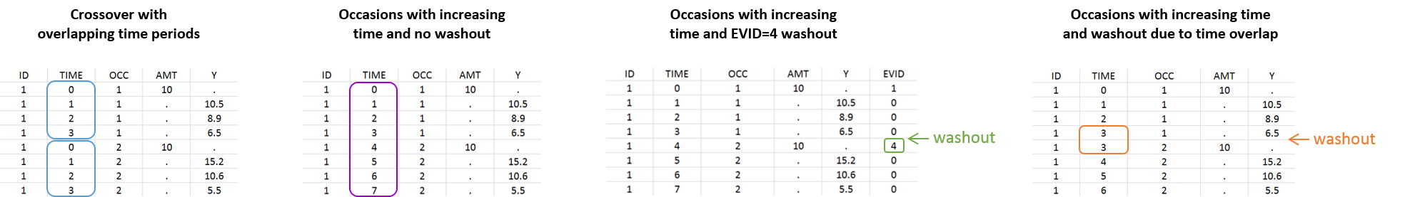
- Cross over study: In that case, data are collected for each patient during two independent treatment periods of time, there is an overlap on the time definition of the periods (e.g both periods start at 0). A column-type OCCASION can be used used to identify the periods. See here for an example.
- Occasions with washout (due to EVENT ID = 4): In that case, there are no overlap between the periods. The time is increasing but the dynamical system (i.e. the compartments) is reset when the second period starts. In particular, EVENT ID = 4 indicates that the system is reset (washout) for example, when a new dose is administrated. See here for an example.
- Occasions with washout (due to overlapping times): In that case, the time is increasing and the overlap between two time points of two different occasions creates a washout. If the washout is not desired, one of the two times can be offset by a small value to avoid the overlap.
- Occasions without washout: In that case, there are no overlap between the periods. The time is increasing and we want to differentiate periods in terms of occasions without any reset of the dynamical system. On the example defined here, multiple doses are administrated to each patient and each period of time between successive doses is defined as a different occasion via the column-type OCCASION.
However, the following situation, which would aim at defining the same occasion index to all morning doses, is not allowed:

How can occasions appear while no OCCASION column is defined?
Occasions are automatically created if there is an EVENT ID column with a value 4, which is not the first record of the individual. Within an individual, each EVENT ID = 4 will create a new occasion. The automatically created occasion column is called OCCevid and will be visible in the Statistical model & Tasks tab in Monolix interface. The data set file itself is not modified (the OCCevid column is internal in Monolix). The OCCevid column is not created if an identical OCCASION column is already present. Inter-occasion variability can be considered for the automatically created OCCevid occasions but doesn’t has to.
The following data on the right has an EVID column (tagged as EVENT ID column-type) with a value of 4. This will automatically create an occasion column called OCCevid. The data set on the left is thus equivalent to the data set on the right:
ID TIME Y EVID 1 0 0 0 1 1 2 0 1 2 2 0 1 0 0 4 1 4 1 0 1 5 2 0 |
ID TIME Y OCCevid 1 0 0 1 1 1 2 1 1 2 2 1 1 0 0 2 1 4 1 2 1 5 2 2 |
|---|
Remark: In MonolixSuite versions prior 2018R1, occasions were also generated by SS=1.
Frequently asked questions on occasions in the data set
- Do all the individual need to share the same sequence of occasion? No, the number of occasions and the times defining the occasions can differ from one individual to another.
- Do the occasion indices need to start at one for each individual? No.
- Do the occasion indices need to be consecutive for each individual? No.
- Is there any limit in terms of number of occasions? No.
- Is it possible to have several levels of occasions? Yes, it can be extended on several level of occasions, see an example here.
Format restrictions
- The OCCASION columns should contain only integers.
- If the OCCASION column-type is used, the OCCASION must be defined for all lines.
2.2.Description of column-types used to time-stamp data
TIME: data time stamp
The TIME columns define the time at wich dose and observation events occurred. When no DATE/DAT1/DAT2/DAT3 column is present, the time represents the time elapsed. When a DATE/DAT1/DAT2/DAT3 column is present, it represents the time of the day. The time can be defined using a double, or a clock format hh:mm or hh:mm:ss. Negative time values are allowed. When the double format is used, and no DATE/DAT1/DAT2/DAT3 column is present, the time has no predefined units. In all other cases, the time units are hours.
When a subject has time under the clock format, all times are converted into relative hours, as on the following example:
| TIME | Reconstructed time | ||
| 10:00 | 10 | ||
| 10:30 | 10.5 | ||
| 14:00 | 14 | ||
| 08:59 | 8.983333 |
When there is no column-type TIME, the column-type NOMINAL TIME is used as time, and if neither TIME nor NOMINAL TIME column-types are present, the column-type DATE is ignored, and the first column-type REGRESSOR is used as time. If no columns are tagged as REGRESSOR, time will be equal to the index of row number containing observations / amounts for each subject-occasion.
Format restrictions
- A data set shall not contain more than one column with the column-type TIME.
- If the TIME column-type is used, the TIME must be defined for all lines.
- String “.” will not be interpreted as a repetition of the previous line and is non-compliant with formats listed here-above.
NOMINAL TIME: data nominal time stamp
The NOMINAL TIME column defines the time at which doses and observations were expected to occur. The column format is the same as the format of the TIME column amd the same restrictions apply, with the exception that lines with missing values are not automatically ignored, but taken from TIME column, if it exists in the data set.
If defined, the NOMINAL TIME column:
- can be used instead of TIME column on x-axis of Observed data (Monolix/PKanalix) and Visual predictive check (Monolix) plots,
- can be used instead of TIME column in the NCA Concentrations table (PKanalix),
- is used in NCA sparse data calculations (PKanalix),
- is used in all other calculations, if TIME column is not defined (Monolix/PKanalix).
DATE/DAT1/DAT2/DAT3: date information
The DATE column-type can be used to indicate the date of the dose or observation event. It is usually used in combination with the TIME column-type, which in that case indicates the time of the day. To accommodate the different date formats, several column types are possible:
| DATE | DAT1 | DAT2 | DAT3 | |
|---|---|---|---|---|
| Day, month and year | mm/dd/yy or mm/dd/yyyy
mm-dd-yy or mm-dd-yyyy |
dd/mm/yy or dd/mm/yyyy
dd-mm-yy or dd-mm-yyyy |
yy/mm/dd or yyyy/mm/dd yy-mm-dd or yyyy-mm-dd |
yy/dd/mm or yyyy/dd/mm yy-dd-mm or yyyy-dd-mm |
By default, when the year is coded with two digits, it is interpreted as 20xx.
Format restrictions
- A data set shall not contain more than one column-type DATE / DAT1 / DAT2 / DAT3.
- Year, day, and month shall be integers.
- The separator must be “/” or “-“
- Character “.” will not be interpreted as a repetition of the previous line and is not compliant with the DATE formats.
- All the lines should be filled correctly within the same delimiter, according to the specified date format: i.e., no empty year, no empty month, no empty day, no mix of delimiters.
Timestamp summary
There are several ways to define the timestamp of the data set depending if there is a TIME column or not and if there is a DATE column or not.
| (NOMINAL) TIME column present | (NOMINAL) TIME column not present | |
| DATE column present | DATE column is considered to represent the day and the TIME column the hour within this day | Date column ignored (regressor or index used) |
| DATE column not present | TIME column is considered to represent the time (no specific units) | First regression-column will be used to timestamp data |
FAQ
- My data is not “over time”, what should I do? You can arbitrarily set the time of each observation to 0.
- What happens if neither TIME nor DATE is defined? We strongly encourage the user to explicitly define the TIME column-type. However, if there is neither TIME nor DATE column-types, the first regression-column (i.e. first column with column-type REGRESSION) will be used to timestamp data. Moreover, if there is no TIME, no DATE and no REGRESSION column-type, time is equal to row indexes of each subject-occasion.
2.3.Description of column-types used to define responses
- OBSERVATION (formerly Y): response
- OBSERVATION ID (formerly YTYPE): response identifier
- CENSORING (formerly CENS): censored observation
- LIMIT: limit for censored values
OBSERVATION (formerly Y): response
The OBSERVATION column-type can be used to record continuous, categorical, count or time-to-event data. For dose lines, the content is free and will not be used. For response lines, the requirements depend on the type of data and are summarized below. Note that the interpretation of dose and response lines has changed between the 2016R1 and the 2018R1 versions, as detailed here.
For continuous data:
The value represents what has been measured (e.g concentrations) and can be any double value.
Examples:
- Basic example:
ID TIME AMT   Y
1   0   50     .
1 0.5    .   1.1
1   1    .   9.2
1 1.5    .   8.5
1   2    .   6.3
1 2.5    .   5.5
- Full data set for continuous data: theophylline data set, the warfarin data set, and the HIV data set
For categorical data:
In case of categorical data, the observations at each time point can only take values in a fixed and finite set of nominal categories. In the data set, the output categories must be coded as consecutive integers.
Examples:
- Basic example:
ID TIME Y
1 0.5   3
1   1   0
1 1.5   2
1   2   2
1 2.5   3
- Full data set for joint continuous and categorical data: warfarin data set.
For count data:
Count data can take only non-negative integer values that come from counting something, e.g., the number of trials required for completing a given task. The task can for instance be repeated several times and the individuals performance followed.
Count data can also represent the number of events happening in regularly spaced intervals, e.g the number of seizures every week. If the time intervals are not regular, the data may be considered as repeated time-to-event interval censored, or the interval length can be given as regressor to be used to define the probability distribution in the model.
Examples:
- Basic example: in the data set below, 10 trials are necessary the first day (t=0), 6 the second day (t=24), etc.
ID TIME  Y
1   0   10
1  24    6
1  48    5
1  72    2
For (repeated) time-to-event data:
In this case, the observations are the “times at which events occur“. An event may be one-off (e.g., death) or repeated (e.g., epileptic seizures, mechanical incidents, strikes). In addition, an event can be exactly observed, interval censored or right censored.
For the formatting of time-to-event data, the column TIME should contain not only the time of an event, but also other relevant times such as the start and end of the observation period or time intervals for interval-censoring. The column OBSERVATION contains an integer that indicates how to interpret the associated time. The different values for each type of event and observation are summarized in the table below:
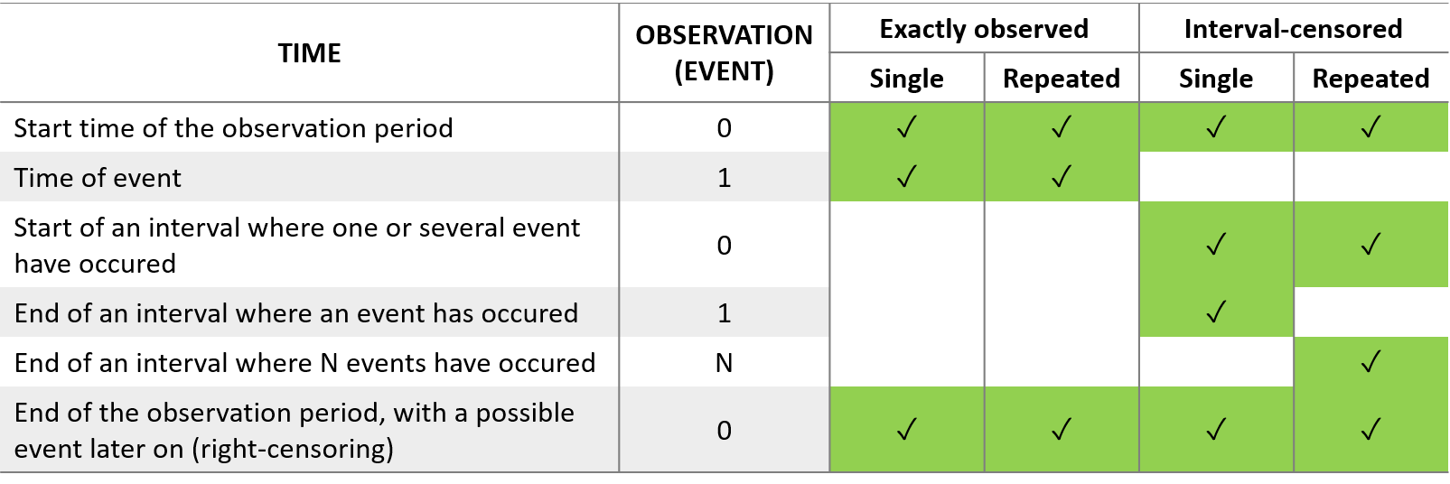
The figure below summarizes the different situations with examples: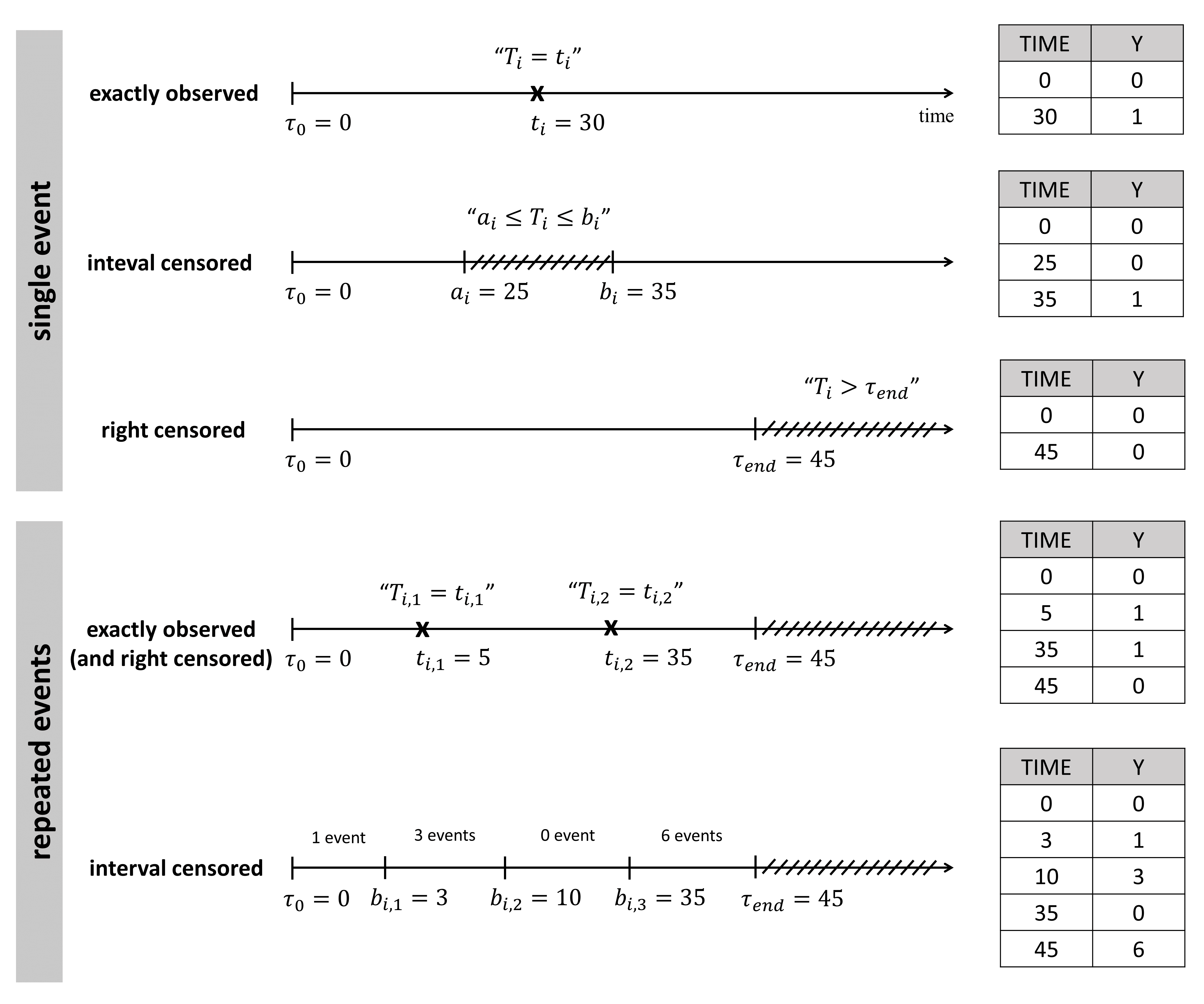
For single events exactly observed:
One must indicated the start time of the observation period with Y=0, and the time of event (Y=1) or the time of the end of the observation period if no event has occurred (Y=0).
Examples:
- Basic example: in the following dataset, the observation period last from starting time t=0 to the final time t=80. For individual 1, the event is observed at t=34, and for individual 2, no event is observed during the period. Thus it is noticed that at the final time (t=80), no event occurred.
ID TIME Y
1   0   0
1  34   1
2   0   0
2  80   0
- Full data sets for time-to-event data: PBC data set and Oropharynx data set
For repeated events exactly observed:
One must indicate the start time of the observation period (Y=0), the end time (Y=0) and the time of each event (Y=1).
Examples:
- Basic example: below the observation period last from starting time t=0 to the final time t=80. For individual 1, two events are observed at t=34 and t=76, and for individual 2, no event is observed during the period.
ID TIME Y
1   0   0
1  34   1
1  76   1
1  80   0
2   0   0
2  80   0
For single events interval censored:
When the exact time of the event is not known, but only an interval can be given, the start time of this interval is given with Y=0, and the end time with Y=1. As before, the start time of the observation period must be given with Y=0.
Examples:
- Basic example: we only know that the event has happened between t=32 and t=35.
ID TIME Y
1   0   0
1  32   0
1  35   1
For repeated events interval censored:
In this case, we do not know the exact event times, but only the number of events that occurred for each individual in each interval of time. The column-type Y can now take integer values greater than 1, if several events occurred during an interval.
Examples:
- Basic example: No event occurred between t=0 and t=32, 1 event occurred between t=32 and t=35, 1 between t=35 and t=50, none between t=50 and t=56, 2 between t=56 and t=78 and finally 1 between t=78 and t=80.
ID TIME Y
1   0   0
1  32   0
1  35   1
1  50   1
1  56   0
1  78   2
1  80   1
Format restrictions
- A data set shall not contain more than one column with column-type OBSERVATION.
- If EVENT ID = 1, 3 or 4, the content of the OBSERVATION column is free and ignored.
- If EVENT ID = 0, and IGNORED OBSERVATION = 1 or 2, the content of the OBSERVATION column is free and ignored.
- If EVENT ID = 0 and IGNORED OBSERVATION = 0, the contant of the OBSERVATION column has to be a double (dots ‘.’ are not allowed).
- If the EVENT ID column is absent (and whatever the IGNORED OBSERVATION column is), the content is free. Values that are not doubles (for instance dots ‘.’ or strings) are ignored.
Warnings
- If a subject or a subject-occasion has no observations, a warning message arises telling which subjects or subjects-occasions have no measurements and will be ignored.
FAQ
- My data is not “over time”, what should I do? You can arbitrarily set the time of each observation to 0.
OBSERVATION ID (formerly YTYPE): response identifier
The OBSERVATION ID column permits to distinguish several types of observations (several concentrations, effects, etc). The OBSERVATION ID column assigns an identifier to each observation of the OBSERVATION column. Those identifiers are used to map the observations of the data set to the outputs of the model (in the OUTPUT block of the Mlxtran model file). The mapping is done following alphabetical order: the first OBSERVATION ID value in alphabetical order is mapped to the first output in the output list, etc. We recommend to use integers (1, 2, …) as identifiers, such that the observations with identifier 1 are mapped to the first output, observations with identifier 2 to the second, etc. If you have more than 10 different outputs, note that in alphabetical order ’10’ become ‘2’. In that case using letters (a, b, c, …) as identifiers is more intuitive. The dot “.” is not considered as a repetition of the previous line but as a different identifier.
There can be more OBSERVATION ID values than there are outputs in the model file. In that case only the observations corresponding to the first identifiers(s) in alphabetical order will be used (example below).
For continuous data, in the Monolix graphical user interface, the data viewer and the plots, the observations will be called yX with X corresponding to the identifier given in the OBSERVATION ID column (for instance y1 and y2 if identifiers 1 and 2 were used in the OBSERVATION ID column).
Examples:
- Basic example with integers: with the following data set
TIME AMT OBS YTYPE
 0   .   12   1
 5   .    6   2
10   .    4   1
15   .    3   2
and the following output block
OUTPUT:
output = {Cc, R}
the observations “12” and “4” which have identifier “1” will be matched to the output “Cc”, while observations ”6″ and “3” with identifier “2” will be matched to “R”.
- Basic example with strings (not recommended): with the following data set
TIME AMT OBS YTYPE
 0   .   12  PK
 5   .    6  PK
10   .    4  PD
15   .    3  PD
and the following OUTPUT block in the Mlxtran model file:
OUTPUT:
output = {Cc, R}
the observations tagged with “PD” will be mapped to the first output “Cc” (which is probably not what is desired), and those tagged with “PK” will be mapped to the second output “R”, because in alphabetical order “PD” comes before “PK”.
- Basic example with more OBSERVATION ID values than model outputs: with the following data set
TIME AMT OBS YTYPE
 0   .   12   1
 5   .    6   2
10   .    4   1
15   .    3   2
and the following output block
OUTPUT:
output = {Cc}
the observations tagged with identifier “1” will be mapped to the model output “Cc” and the observations tagged with “2” will be ignored. If the user wants to use only the data tagged with “2”, he can add an IGNORED OBSERVATION column which ignores all observations with identifier “1” (see below).
- Basic example with more OBSERVATION ID values than model outputs and an IGNORED OBSERVATION column: with the following data set
TIME AMT OBS YTYPE MDV
 0   .   12   1     1
 5   .    6   2     0
10   .    4   1     1
15   .    3   2     0
and the following output block
OUTPUT:
output = {Cc}
the observations tagged with identifier “1” will all be ignored (due to the MDV column tagged as IGNORED OBSERVATION) and the observations with identifier “2” will be mapped to the model output “Cc”.
- Full data set example: warfarin PKPD data set, PSA and survival data set
Format restrictions:
- A data set shall not contain more than one column with column-type OBSERVATION ID.
- The content of the OBSERVATION ID column can be strings or integers.
- The dot “.” is not considered as a repetition of the previous line but as a different identifier.
CENSORING (formerly CENS): censored observation
The CENSORING column permits to mark censored data. When an observation is marked as censored, the (upper or lower) limit of quantification is given in the OBSERVATION column (not in a separate column).
- CENSORING = 1 means that the value in OBSERVATION column (that we call \(y_{obs}\) here) is an upper limit. The true observation y verifies \(y<y_{obs}\).
- CENSORING = 0 means the value in response-column corresponds to a valid observation (no interval associated).
- CENSORING = -1 means that the value in OBSERVATION column (\(y_{obs}\)) is a lower bound. The true observation y verifies \(y>y_{obs}\).
The mathematical handling of censored data is described here.
Format restrictions:
- A data set shall not contain more than one column with column-type CENSORING.
- For dose lines, the content is free and will be ignored.
- For response lines, there are only four possible values : -1, 0, 1 and ‘.’ (interpreted as 0).
LIMIT: limit for censored values
When the column LIMIT contains a numeric value and CENSORING is different from 0, the value in the LIMIT column is interpreted as the second bound of the interval. Writing \(y_{obs}\) the value in the OBSERVATION column and \(y_{limit}\) the value in the LIMIT column, the true observation y verifies \(y\in [y_{limit}, y_{obs}]\). When LIMIT = ‘.’ , the value is interpreted as -infinity or +infinity depending on the value of CENSORING (1 or -1 respectively) as if the LIMIT column would not be present.
Format restrictions:
- A data set shall not contain more than one column with column-type LIMIT.
- A data set shall not contain any column with column-type LIMIT if no column with column-type CENSORING is present.
- Allowed values are doubles and dot ‘.’ , and strings are not allowed (even when CENSORING = 0).
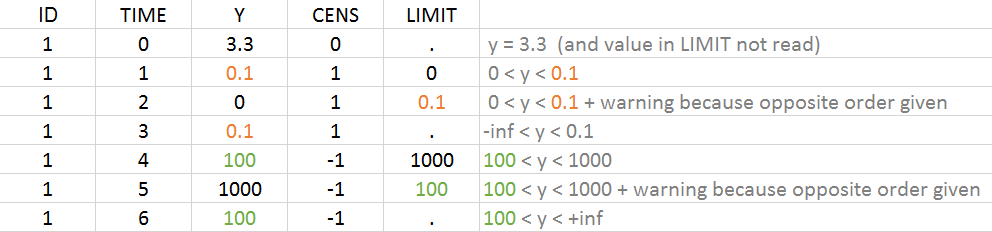
Example with CENSORING and LIMIT
It is possible to have both censoring type on the same individual, i.e. both upper or lower limit of quantification. It is possible to have measurements with and without bounds. The example below gives an overview of the possible combinations:
2.4.Description of column-types used to define the dose regimen
AMOUNT (formerly AMT): dose amount
The AMOUNT column records the amount of the administrated doses. For dose-lines, the value must be a double. For response-lines, the content is free. Note that the interpretation of dose and response lines has changed between the 2016R1 and the 2018R1 versions, as detailed here.
Examples:
- Basic example: the individual 1 receives a dose of 10 at time 0
ID  TIME  AMT  Y
1    0    10   .
1    1     .   6
1    2     .   4
- Example with a single dose split into two routes of absorption: a single dose may be absorbed at different sites, leading to several absorption route. This can be taken into account by splitting the dose into several fractions, directed to several absorption macros. With the following data set:
ID  TIME  AMT  Y
1    0    10   .
1    1     .   6
1    2     .   4
and the following PK block in the model file:
PK:
oral(ka=ka1, p=F)
oral(ka=ka2, Tlag, p=1-F)
a fraction F of the dose is absorbed via a first-ordre process with rate constant ka1, and a fraction 1-F is absorbed with a absorption constant ka2 after a lag time Tlag.
Format restrictions:
- A data set shall not contain more than one column-type AMOUNT.
- For dose-lines with EVENT ID = 1, 3 or 4, the value must be a double.
- For lines without EVENT ID, the value must be a double or a dot ‘.’
ADMINISTRATION ID (formerly ADM): administration identifier
The ADMINISTRATION ID column permits to distinguish different types of administrations, for instance oral administrations and intravenous administrations. The content of the ADMINISTRATION ID column is used for dose-line only and must be a positive integer. This integer works like a flag, which can be used in the model file to link the dose informations of the data set to a specific administration route in the model.
Examples:
- Example with oral and iv administrations: For instance, with the following data set:
ID  TIME AMT ADM Y
John 0   10   1  .
Eric 0   20   2  .
Jean 0   10   3  .
and the following PK block in the Mlxtran model file:
PK:
iv(adm=1)
oral(adm=2, ka)
the subject John will receive a dose of 10 via a bolus iv, while subject Eric will receive a dose of 20 orally with first-order rate constant ka. The identifier in the ADMINISTRATION ID column should match the “adm=” field of the administration macros. A same subject can receive some doses via one route and other doses via another route. The administration type with id ‘3’ is not used in the model, thus all doses with this id will not be applied.
The default value for administration types is 1. This means that if there is no column ADMINISTRATION ID in the dataset, all doses will be associated to the administration id 1. If the dataset contains a column ADMINISTRATION ID but the structural model does not include arguments adm to indicate how to apply the different types of doses, only the doses with administration id ‘1’ in the data set will be used.
Changes compared to the 2016R1 version: In the 2016R1 version the ADM column could be used simultaneously as administration identifier for dose-lines and as observation identifier for response-lines. In the 2018R1 version the ADMINISTRATION ID column is used only for dose lines.
Format restrictions:
- For dose-lines, the column shall contain only positive integers. For response-lines, dots ‘.’ or integers are allowed.
- A data set shall not contain more than one ADMINISTRATION ID column-type.
INFUSION RATE and INFUSION DURATION (formerly RATE and TINF): rate and duration of infusion
These columns enable to define the rate (INFUSION RATE column-type) or duration (INFUSION DURATION column-type) of doses administered as infusions. The column content is meaningful only for dose-lines. The rate and duration information is transferred to the model via the use of the iv macro, depot macro or pkmodel macro. If a RATE is defined, the duration of the infusion will be AMOUNT/RATE. If a DURATION is defined, the rate will be AMOUNT/DURATION. The units must be coherent with the units of the AMOUNT and TIME columns. A dose-lines, if a negative value, or dot ‘.’ or 0 is used, the infusion will be replaced by a bolus.
We strongly recommend to have small duration values (less than 10). Indeed, if the duration is too long, the calculation of the analytical solution of the model may produce NaN. Two workarounds are possible:
– Either rescale the time units to have smaller duration values.
– Use ODEs instead of analytical solutions. ODEs can be enforced with useAnalyticalSolution = no in the model file.
Examples:
- Basic example: with the following data set, assuming the TIME units are minutes and AMOUNT units mg, an amount of 10 mg will be applied via an infusion over 5 minutes starting at time 0. This is equivalent to a RATE of 2 mg/minute. The 20 mg doses at time 2, 3, and 4 minutes are applied via a bolus.
ID  TIME  AMT  TINF Y
1    0    10    5   .
1    1     .    .   6
1    2    20    0   .
1    3    20   -2   .
1    4    20    .   .
Format restrictions:
- A data set shall not contain more than one column with column-type INFUSION RATE or INFUSION DURATION.
- A negative value, “.” or 0 means a bolus dose, without any infusion rate or time.
- For dose-lines, the value must be a double, or a dot ‘.’.
- For response lines, the content is free.
STEADY STATE and INTERDOSE INTERVAL (formerly SS and II): steady-state and inter-dose interval
Steady-state is used to specify that any transitory effect is over and that the system response is now a periodic function of doses. In practice, a fixed number of doses (by default 5) is added before the dose entered with the STEADY STATE flag (so 6 doses in total, by default). The period between doses is set to the INTERDOSE INTERVAL. The number of doses to add can be changed when loading the data and will be saved in the project file. The number of added doses may be reduced compared to the specified value if the doses to add would interfere with another dose or observation: any steady-state dose that would be added before (i.e earlier in time) a dose or response line is not added, even if the line information is ignored (for instance with EVENT ID = 2 or IGNORED OBSERVATION = 1).
The allowed values are the following:
- STEADY-STATE = 0 or ‘.’ : no steady-state, the dose is a normal dose.
- STEADY-STATE = 1 : the system has achieved steady-state. A washout (i.e reset to the initial values of the model) is applied before the first added dose.
- STEADY-STATE = 2 or 3 : the system has achieved steady-state. Unlike STEADY-STATE = 1, no washout is added.
STEADY-STATE and EVENT ID: when STEADY-STATE = 1 is used on the same line as EVENT ID = 3 or 4, a washout is applied just before the first dose added for steady-state (because of STEADY-STATE = 1) and also just before the dose defined on that line (because of EVENT ID = 3 or 4). When STEADY-STATE = 2 or 3 is used on the same line as EVENT ID = 3 or 4, a washout is added just before the dose defined on that line.
STEADY-STATE and REGRESSOR: see the REGRESSOR page.
Changes with respect to the MonolixSuite2016R1 version:
- In versions prior MonolixSuite2018R1, the number of added doses can be changed in the preferences.xmlx file, located in
<home>/lixoft/monolix/configin the user folder. By default, the number of doses is 5 and was defined in the line<dosesToAddForSteadyState value="5"/>.It can for instance be changed to<dosesToAddForSteadyState value="20"/>. - In versions prior MonolixSuite2018R1, SS=1 was generating new occasions. This is not the case anymore.
- In versions prior MonolixSuite2018R1, SS=2 and SS=3 were not allowed.
Examples:
- Basic example: On the following example:
ID TIME AMT SS II  Y
1   0    10  1  2  .
5 doses are applied, at times -10, -8, -6, -4, -2 in addition to the dose at time = 0. The above data set is thus equivalent to:
ID TIME AMT SS II  Y
1  -10  10  0  0   .
1   -8  10  0  0   .
1   -6  10  0  0   .
1   -4  10  0  0   .
1   -2  10  0  0   .
1    0  10  0  0   .
The first added dose will have a wash-out.
- Example with informations colliding with doses to add: The following data set, with a normal dose at t=0 and a steady-state dose at t=10 with an interdose-interval of 3.5 will lead to the following situation:
ID TIME Y AMT SS II 1 0 . 10 0 0 1 0 10 . . . 1 1 6 . . . 1 2 4 . . . 1 10 . 10 1 3.5 1 11 9 . . . 1 12 6 . . . 1 13 3 . . . 1 14 2 . . . |
 |
Even if 5 additional doses are specified in the GUI when loading the data, there will be only 2 additional doses as otherwise the previous measurements would be interfered with. In addition, there is a washout (highlighted in purple) just before the first added dose.If we would replace SS=1 by SS=2 on line 5, we would again have only 2 doses added but no wash out as can be seen in the following figure:
ID TIME Y AMT SS II 1 0 . 10 0 0 1 0 10 . . . 1 1 6 . . . 1 2 4 . . . 1 10 . 10 2 3.5 1 11 9 . . . 1 12 6 . . . 1 13 3 . . . 1 14 2 . . . |
 |
- Typical example with pre-dose PK measurement, dose at site and post-dose PK measurements: the subject takes regularly doses at home. During a hospital visit, he gets a pre-dose PK measurement, a dose at site, and one or several post-dose PK measurements. The STEADY-STATE statement cannot be applied on the dose administered at site, as the doses to add would interfere with the pre-dose PK measurement. We thus need to write:
ID TIME  AMT  SS  II    Y
1   0     10   1  24    .     ; steady-state statement
1  23.9    .   .   .   5.5    ; pre-dose measurement
1  24     10   .   .    .     ; dose at site
1  25      .   .   .   9.9    ; post-dose measurement
FAQ:
- Can I define two different STEADY-STATE lines for morning and evening doses? No, as the doses to add would collide with each other. You will have to use an ADDITIONAL DOSES column instead.
Format restrictions for STEADY-STATE:
- A data set shall not contain more than one column with column-type STEADY STATE.
- If there is a column-type STEADY STATE, there should be a column-type INTERDOSE INTERVAL.
- Accepted values (for all lines, including response-lines): 0, 1, 2, 3 or dot ‘.’
Format restrictions for INTERDOSE-INTERVAL:
- A data set shall not contain more than one column with column-type INTERDOSE INTERVAL.
- If there is a column-type STEADY STATE, there should be a column-type INTERDOSE INTERVAL.
- Accepted values:
- on response-line: 0 or ‘.’ (non-zero double value will generate a warning)
- on normal dose-line (no STEADY-STATE or ADDITIONAL DOSE): 0 or ‘.’ (non-zero double value will generate a warning)
- on STEADY-STATE or ADDITIONAL DOSE line: non-zero double value
- Clock format is not accepted
ADDITIONAL DOSES (formerly ADDL): additional dose line
The ADDITIONAL DOSES column is a useful shortcut to specify dose regimens with repetitive treatments. The value in ADDITIONAL DOSES is the number of times the dose shall be repeated (in additional to the dose defined on that line) and column INTERDOSE INTERVAL contains the dose repetition interval. Doses that would be added after the last measurement are useless and will thus not be added.
ADDITIONAL DOSES and REGRESSOR: see the REGRESSOR page.
Examples:
- Basic example: For instance to specify a dose of 10 every 12 hours during 3 days it is possible to write:
ID TIME AMT
Tom  0  10
Tom 12  10
Tom 24  10
Tom 36  10
Tom 48  10
Tom 60  10
Tom 72  10
but ADDITIONAL DOSES (ADDL) and INTERDOSE INTERVAL (II) can also be used to specify the same information in a single line
ID TIME AMT ADDL II
Tom  0   10   6  12
Format restrictions:
- When there is an ADDL column there must be an INTERDOSE INTERVAL (interdose interval) column to indicate the inter dose timing.
- For dose-lines with ADDL strictly positive, the INTERDOSE INTERVAL value must be strictly positive.
- Accepted values:
- on normal dose lines: 0 or ‘.’
- on response lines: 0 or ‘.’
- on lines where ADDITIONAL DOSES is needed: positive integer
2.5.Description of column-types used to define covariates
CONTINUOUS COVARIATE (formerly COV): continuous covariate
The column-type CONTINUOUS COVARIATE is used to tag continuous covariates, i.e covariates which can take values on a continuous scale (such as weight or age). Covariates tagged in the data set can (but don’t have to) be used as covariates in the model. The covariate value must be constant within subjects (or within occasions if occasions are present). If the value is not constant, the first value of each subject in time ordering will be used for all times (and a warning is generated). To define time varying covariate, use REGRESSORS (example here).
The allowed values are doubles or dot ‘.’. There must be at least one non-dot value per subject (or per occasion if occasions are defined).
Examples:
- Basic example: in the following data set, individual 1 has weight WT = 78, individual 2 has WT = 80 for all times points (first value in time ordering) and individual 3 has WT = 90.
ID  TIME  Y    WT
1    0   5.7   78
1    1   5.6   78
2    0   6.7   80
2    1   6.5   82
3    0   7.8    .
3    1   8.9   90
Format restrictions:
- Continuous covariate columns shall contain either a double or “.”.
- The covariate must be defined at least once per subject-occasion.
- The covariate must remain the same for all the lines within the same subject-occasion.
CATEGORICAL COVARIATE (formerly CAT): categorical covariate
The column-type CATEGORICAL COVARIATE is used to tag categorical covariates, i.e covariates which can only take a finite number of values (such as sex or a genotype). Covariates tagged in the data set can (but don’t have to) be used as covariates in the model. The covariate value must be constant within subjects (or within occasions if occasions are present). If the value is not constant, the first value of each subject in time ordering will be used for all times (and a warning is generated). To define time varying covariate, use REGRESSORS (example here).
The allowed values are strings, doubles or dot ‘.’. There must be at least one non-dot value per subject (or per occasion if occasions are defined), otherwise the category is considered to be ‘NA’.
Examples:
- Basic example: in the following data set, the covariate SEX has two categories ‘F’ and ‘M’ and the individual 3 has value ‘F’. The covariate GENO has three categories ‘1’, ‘2’ and ‘NA’ (coming from the individual 3 which has no valid value). The covariate RACE has only one category ‘1’. Individual 1 has RACE = 1, as this is the value defined first in time. RACE will not appear in the graphical user interface because it is not possible to use a covariate with only one category in a model.
ID  TIME  Y  SEX GENO RACE
1    0   5.7  F   1     1
1    1   5.6  F   1     2
2    0   6.7  M   2     1
2    1   6.5  M   2     1
3    0   7.8  .   .     1
3    1   8.9  F   .     1
Format restrictions:
- The covariate must be defined at least once per subject-occasion.
- The categorical covariate must be the same for all the lines with the same subject-occasion.
2.6.Description of column-types used to define regressions
REGRESSOR (formerly X): regression value
REGRESSOR columns define variables (possibly time-varying) that will be available for calculations in the structural model after regressor definition. Regressors can for instance be used to take into account time-varying covariates (example here), or tag the columns corresponding to individual PK parameters in a sequential PKPD modeling approach.
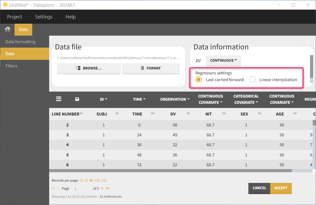
Allowed values in the REGRESSOR column are doubles and dot ‘.’ (to indicate missing values). For the first record (observation or dose line) of each subject (or subject-occasion if occasions are present), the regressor value cannot be missing (no dot ‘.’ allowed). For the following missing values, the interpolation will be done using the setting chosen in the GUI, which can be “Last Carried Forward” or “linear interpolation”. Regressor values on observation or dose lines are used the same way, as well as regressor values on lines with no observation and no dose.
- last carried forward: if we have defined in the dataset two times for each individual with (reg_A) at time (t_A) and (reg_B) at time (t_B)
- for (tle t_A), (reg(t)=reg_A) [first defined value is used]
- for (t_Ale t<t_B), (reg(t)=reg_A) [previous value is used]
- for (t>t_B), (reg(t)=reg_B) [previous value is used]
- linear interpolation: the interpolation is:
- for (tle t_A), (reg(t)=reg_A) [first defined value is used]
- for (t_Ale t<t_B), (reg(t)=reg_A+(t-t_A)frac{(reg_B-reg_A)}{(t_B-t_A)}) [linear interpolation is used]
- for (t>t_B), (reg(t)=reg_B) [previous value is used]
Several columns can be tagged as REGRESSOR. In that case, the mapping with the regressors defined in the model is done by name if possible, otherwise by order: the first column tagged as REGRESSOR in the data set is mapped to the first element in the model input list defined as regressor.
If within a subject (or subject-occasion if occasions are present) two events are defined at the same time on two different lines, the regressor value must be the same on both lines. The regressor value is used even if the dose or observation is ignored (for instance using the EVENT ID and IGNORED OBSERVATION columns).
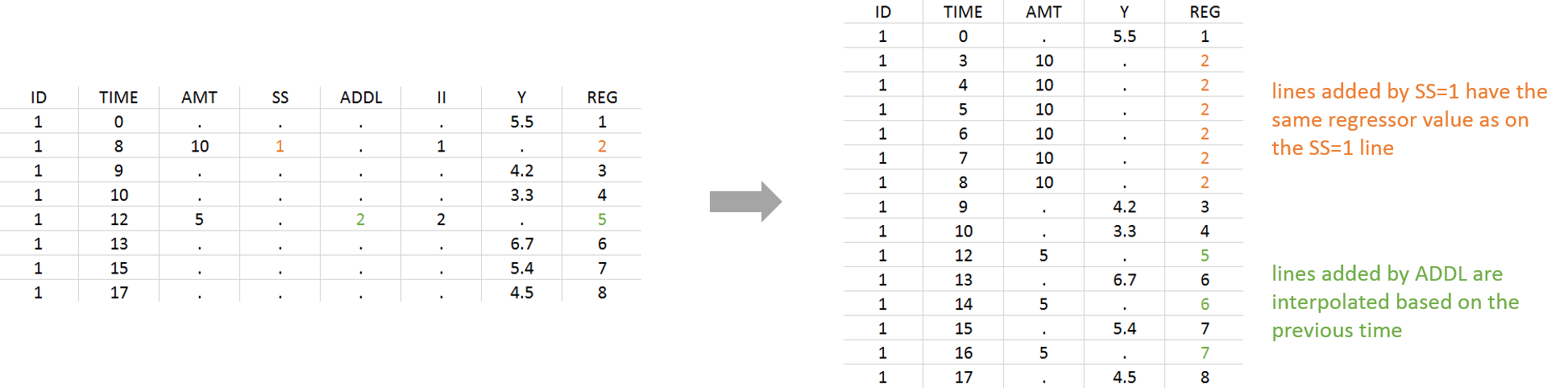
Lines added due to a STEADY-STATE column get the same regressor value as the line with the STEADY-STATE statement. Lines added due to an ADDITIONAL DOSES column get a dot ‘.’ and are then interpolated based on the previous values.
Examples:
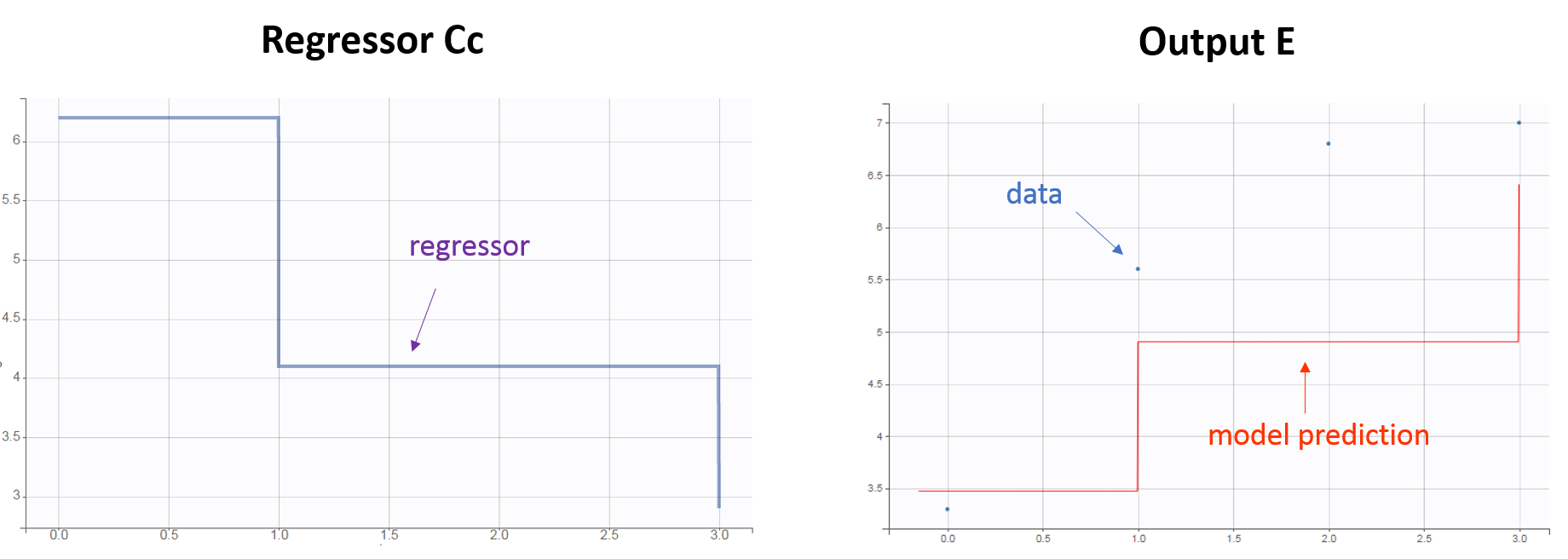
- Example with one regressor: the regressor corresponds to the drug concentration, which will be used in a direct effect PD model. With the following data set:
ID  TIME  Y    REG
1     0  3.3   6.2
1     1  5.6   4.1
1     2  6.8    .
1     3  7.0   2.9
and the following model:
[LONGITUDINAL]
input = {E0, IC50 , Cc}
Cc = { use = regressor }

EQUATION:
E = E0 * (1 - Cc/(Cc+IC50))

OUTPUT:
output = {E}
The regressor variable Cc in the model will take the values defined in the REG column and be used to calculate the effect E. For time points not defined in the data set, interpolation will be done depending on the chosen Regressor Setting. If “Last Observation Carried Forward” is selected: during the time interval [0, 1[, the regressor value is that defined on time 0. Note that the column header and the model regressor variable name can differ.
- Example with two regressors: the regressors correspond to the individual PK parameters used to calculate the drug concentration, itself impacting the effect E. With the following data set:
ID  TIME  AMT  Y    V_mode  k_mode
1     0   10   .     6.2     1.2
1     0    .  3.3    6.2     1.2
1     1    .  5.6    6.2     1.2
1     2    .  6.8    6.2     1.2
1     3    .  7.0    6.2     1.2
and the following model:
[LONGITUDINAL]
input = {E0, EC50 , V, k}
V = { use = regressor }
k = { use = regressor }

EQUATION:
Cc = pkmodel(V,k)
E = E0 * (1 - Cc/(Cc+EC50))

OUTPUT:
output = {E}
The first column tagged as REGRESSOR (V_mode) is mapped to the first regressor in the input list (V), and the REGRESSOR column of the data set (k_mode) is mapped to the second regressor of the model (k).

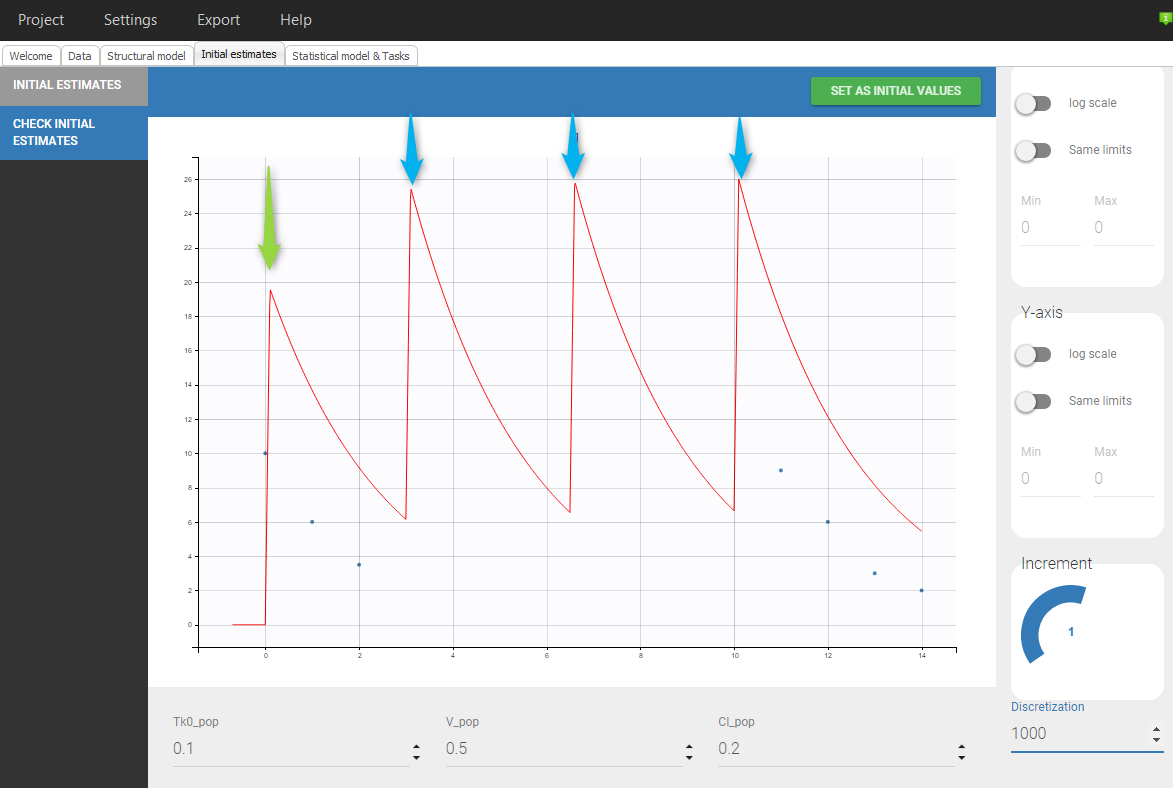
- Example with STEADY-STATE and ADDITIONAL DOSES:
Format restrictions:
- The regression-columns (i.e. columns with column-type REGRESSOR) shall contain either doubles or “.” (which will be interpolated).
- The first record for each subject (or subject-occasion) cannot be dot ‘.’ .
- When there are several lines with the same time, same id and same occasion, the value of the regressor column must be the same.
2.7.Description of column-types used to define controls and events
- EVENT ID (formerly EVID): event identification
- IGNORED OBSERVATION (formerly MDV): ignores the observations
- IGNORED LINE: ignores all the element of the line
EVENT ID (formerly EVID): event identification data item.
The EVENT ID column permits to assign lines to be dose or response-lines, and to define washouts/resets. The column is not mandatory, as dose and response lines can be recognized based on the content (see here for details). The EVENT ID column can take 5 different values:
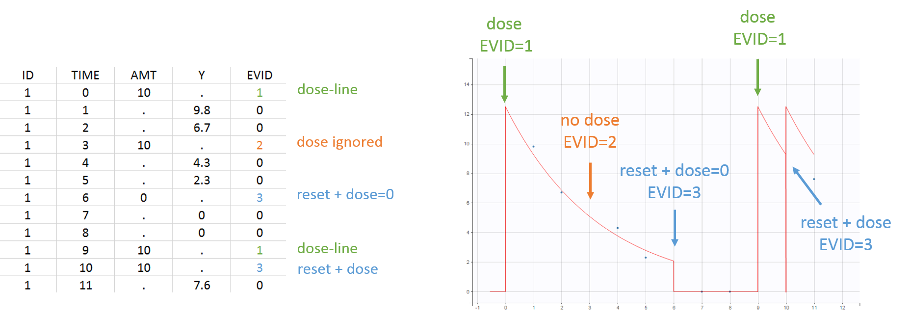
- EVENT ID = 0: observation event, the line is a response-line. The dose-related informations (AMOUNT column, etc) are ignored.
- EVENT ID = 1: dose event, the line is a dose-line. The response-related informations (OBSERVATION column, etc) are ignored.
- EVENT ID = 2: other event. Both the dose information and the observation are ignored. Note that no prediction will be outputted for that time in the output files.
- EVENT ID = 3: reset + dose event. The system is reset to the initial values and the dose is applied immediately after. To do a reset without applying a new dose, the dose amount can be set to zero. Unlike EVENT ID = 4, no occasions are created. The line is a dose-line (i.e the response-related informations are ignored).
- EVENT ID = 4: reset + dose event. The system is reset to the initial values and the dose is applied immediately after. If at least one EVENT ID = 4 appear at a position which is not the first record of an individual, a OCCASION column-type called OCCevid will be created. It may (but doesn’t have to) be used to define inter-occasion variability. To do a reset without applying a new dose, the dose amount can be set to zero. The line is a dose-line (i.e the response-related informations are ignored).
All combinations of EVENT ID and IGNORED OBSERVATION values are possible and EVENT ID has priority over IGNORED OBSERVATION (for instance if EVENT ID = 1 and IGNORED OBSERVATION = 0, the line is a dose-line). For all EVENT ID values, the REGRESSOR values are taken into account.
Examples:
- Example with EVENT ID = 0, 1, 2 and 3:
- Example with EVENT ID = 4:

Format restrictions:
- A data set shall not contain more than one column with column-type EVENT ID.
- EVENT ID shall contain an integer in {0, 1, 2, 3, 4}.
- When a line is tagged EVENT ID = 0, and IGNORED OBSERVATION = 0, the value contained in column OBSERVATION shall be a double.
- When a line is tagged EVENT ID = 1, 3 or 4, the value in the AMOUNT column shall be a double.
IGNORED OBSERVATION (formerly MDV): ignores the observations (missing dependent variable).
The IGNORED OBSERVATION column-type enables to tag lines for which the information in the OBSERVATION column-type should be ignored (because they are outliers, or because one wants to ignore all PK measurements for instance). The column is not mandatory. Several IGNORED OBSERVATION columns are possible (see below) and 3 values are possible:
- IGNORED OBSERVATION = 0: the value in the OBSERVATION column is not ignored. If in addition EVENT ID = 0, the value in the OBSERVATION column has to be a double.
- IGNORED OBSERVATION = 1: the value in the OBSERVATION column is ignored.
- IGNORED OBSERVATION = 2: identical to IGNORED OBSERVATION = 1. Note that no prediction will be made at that time point in the output files.
If there are both an IGNORED OBSERVATION and an EVENT ID column, the EVENT ID column has priority to define dose and response-lines (see here for more details). It is not necessary to set IGNORED OBSERVATION = 1 when EVENT ID = 1.
For all IGNORED OBSERVATION values, the REGRESSOR values are taken into account.
It is possible to have multiple IGNORED OBSERVATION columns in order to ignore observations for different reasons (for instance an “outliers” column to ignore outliers and a “placebo” column to ignore individuals which received only placebo, both tagged as IGNORED OBSERVATION column-type). When there are multiple IGNORED OBSERVATION columns, a synthetic value is computed as:
- if IGNORED OBSERVATION = 0 in all columns, then resulting synthetic IGNORED OBSERVATION equals 0.
- if IGNORED OBSERVATION = 1 or 2 in at least one column, then the resulting synthetic IGNORED OBSERVATION equals 1.
Examples:
- Example with IGNORED OBSERVATION = 0, 1 or 2:

Format restrictions:
- IGNORED OBSERVATION shall contain only integers in {0, 1, 2}.
- If IGNORED OBSERVATION = 0 and EVENT ID = 0, the value in the OBSERVATION column has to be a double.
IGNORED LINE: ignores all the element of the line
Starting from the 2019 version, the IGNORED LINE column-type enables to tag lines for which all the information should be ignored (because they are outliers, or because one wants to ignore all PK measurements for instance). Contrary to the IGNORED OBSERVATION column-type that only ignores the observation value, the IGNORED LINE column-type allows to ignore doses and regressor values in addition to the observation values.
The column is not mandatory.
Starting from the 2021 version, there can be several columns IGNORED LINE, while in previous versions there can be only one such column.
Starting from the 2024 version, IGNORED LINE column can contain integers larger than 1, while previously the values were restricted to 0 and 1.
Format restrictions:
- IGNORED LINE shall contain only non-negative integers.
2.8.Character definition
Character definition
We recommend to use only alphanumeric characters and the underscore “_” character in the strings of your data set.
Unfortunately, in the Monolix2016R1 suite, special characters such as spaces ” “, stars “*”, parentheses “(“, brackets “[“, dashes “-“, dots “.” and slashes “/” are not supported in:
- The headers
- The strings in CAT column.
Please be careful that if your data set includes unsupported characters, the error will only de detected and displayed when loading a saved project (and not when creating and saving the project).
This feature is back in MonolixSuite2018R1.
On the use of “.”
The “.” can be used in almost all the lines of the data set but has several meaning depending on the context. The following table summarizes the use of it.
| Type of column | Not allowed | Considered as a regular string | Considered as | Not considered |
| ID | X | |||
| OCCASION (OCC) | X | |||
| TIME | X | |||
| DATE/DAT1/DAT2/DAT3 | X | |||
| OBSERVATION (Y) | On a response line | On a dose line | ||
| OBSERVATION ID (YTYPE) | On a response line | On a dose line (not read) | ||
| CENSORED (CENS) | 0 | |||
| LIMIT | -Inf if CENS =1 , +Inf if CENS = -1 | |||
| AMOUNT (AMT) | On a dose line | On a response line (not read) | ||
| ADMINISTRATION ID (ADM) | On a dose line | On a response line (not read) | ||
| STEADY STATE (SS) | 0 | |||
| ADDITIONAL DOSE (ADDL) | 0 | |||
| INTERDOSE INTERVAL (II) | 0 | |||
| CONTINUOUS COVARIATE (COV) | Previously defined value of the COV (in the ID/OCC) | |||
| CATEGORICAL COVARIATE (CAT) | X | |||
| REGRESSOR | Interpolation | |||
| EVENT ID (EVID) | X | |||
| IGNORED OBSERVATION (MDV) | X |
3.Data set examples
This section presents several data sets to show some concrete data set and see how to integrate censored data, covariates, …
Data sets with continuous outputs
- Theophylline data set: continuous outputs are taken into account along with categorical and continuous covariates (sex and weight respectively). Moreover, censored data are also managed.
- Tobramycin data set: continuous PK output are taken into account, along with categorical and continuous covariates.
- HIV data set: two continuous censored outputs are considered. No dose is used in the data set, and the treatment type is considered as a categorical covariate.
- Veralipride data set: continuous output with an interesting absorption variability being by far the most probable physiological explanation for the double peak phenomenon.
-
Remifentanil data set: Remifentanil is an opioid analgesic drug with a rapid onset and rapid recovery time. Remifentanil concentration over 65 healthy adults is proposed.
Data sets with discrete count outputs
- Epilepsy attacks data set: count outputs are taken into account along with categorical and continuous covariates. The data arose from a clinical trial of 59 epileptics who were randomized to receive either the anti-epileptic drug progabide or a placebo, as an adjuvant to standard chemotherapy. Patients attended four successive post-randomisation clinic visits, where the number of seizures that occurred over the previous 2 weeks was reported.
- Crohn’s Disease Adverse Events data set: Data set issued from a study of the adverse events of a drug on 117 patients affected by Crohn’s disease (a chronic inflammatory disease of the intestines). In addition to the response variable number of adverse events, 7 explanatory variables were recorded for each patient.
Data sets with discrete categorical outputs
- Respiratory status data set: the respiratory status of patients under placebo or treatment is categorized as “poor” or “good” once per month during 5 months over 111 patients.
- Inpatient multidimensional psychiatric data set: categorical output with a categorical covariate (treatment) during 6 weeks. These data are from the National Institute of Mental Health Schizophrenia Collaborative Study and are available here. Patients were randomized to receive one of four medications, either placebo or one of three different anti-psychotic drugs. The primary outcome is item 79 on the Inpatient Multidimensional Psychiatric.
- Zylkene data set: The putative effects of a tryptic bovine αs1-casein hydrolysate on anxious disorders in cats was investigated using this data set over 24 cats. The score is a global score of emotional state.
Data sets with time-to-event outputs
- PBC data set: PBC is a rare but fatal chronic liver disease of unknown cause, with a prevalence of about 50-cases-per-million population. Between January, 1974 and May, 1984, the Mayo Clinic conducted a double-blinded randomized trial in primary biliary cirrhosis of the liver (PBC), comparing the drug D-penicillamine (DPCA) with a placebo.
- Veterans’ Administration Lung Cancer data set: In this study conducted by the US Veterans Administration, time to death was recorded for 137 male patients with advanced inoperable lung cancer, which were given either a standard therapy or a test chemotherapy.
- NCCTG lung cancer data set: The North Central Cancer Treatment Group (NCCTG) data set records the survival (time-to-event output) of 228 patients with advanced lung cancer, together with assessments of the patients performance status measured either by the physician and by the patients themselves.
- Cardiovascular data set: A subset of the fields was selected to model the differential length of stay for patients entering the hospital to receive one of two standard cardiovascular procedures: CABG and PTCA. The data set contains 3589 individuals.
Joint data sets
- Warfarin data set: Warfarin is an anticoagulant normally used in the prevention of thrombosis and thromboembolism. Plasma warfarin concentrations and Prothrombin Complex Response in thirty normal subjects after a single loading dose are measured. Both measurements are continuous.
- Remifentanil data set: Remifentanil is an opoid analgesic drug with a rapid onset and rapid recovery time. Both remifentanil concentration and EEG measurement are proposed on 65 healthy adults. Both measurements are continuous.
- PSA and survival data set: PSA kinetics and survival data for 400 men with metastatic Castration-Resistant Prostate Cancer (mCRPC) treated with docetaxel and prednisone, the first-line reference chemotherapy, which constituted the control arm of a phase 3 clinical trial. In this context of advanced disease, the incidence of death is high and the PSA kinetics is closely monitored after treatment initiation to rapidly detect a breakthrough in PSA and propose rescue strategies.
3.1.Data sets with continuous outputs
3.1.1.Theophylline data set
Theophylline data set
The data considered here are courtesy of Dr. Robert A. Upton of the University of California, San Francisco. Theophylline is a methylxanthine drug used in therapy for respiratory diseases such as chronic obstructive pulmonary disease (COPD) and asthma under a variety of brand names. Theophylline was administered orally to 12 subjects whose serum concentrations were measured at 11 times over the next 25 hours. This is an example of a laboratory pharmacokinetic study characterized by many observations on a moderate number of individuals. A representation of the concentration over time for each subject is presented on the following figure (notice, that this figure was generated using Datxplore).
 The purpose of this page is to see the construction, the definition and the use of such a data set in Datxplore and Monolix. For sake of simplicity, we look only on one subject (corresponding to ID 1).
Simplified data set
The data set for subject one writes as follows
ID AMT TIME    CONC    WEIGHT  SEX
1   4.02    0   .   79.6    M
1   .   0.25    2.84    79.6    M
1   .   0.57    6.57    79.6    M
1   .   1.12    10.5    79.6    M
1   .   2.02    9.66    79.6    M
1   .   3.82    8.58    79.6    M
1   .   5.1 8.36    79.6    M
1   .   7.03    7.47    79.6    M
1   .   9.05    6.89    79.6    M
1   .   12.12   5.94    79.6    M
1   .   24.37   3.28    79.6    M
Interpretation
One can see the following columns
- ID: the subject ID, column-type ID.
- AMT: the amount of drug provided to this subject, column-type AMOUNT.
- TIME: the time of the event, column-type TIME.
- CONC: the measured concentration, column-type OBSERVATION.
- WEIGHT: Weight of the subject, column-type CATEGORICAL COVARIATE.
- SEX: Sex of the subject, column-type CATEGORICAL COVARIATE.
Several points can be noticed.
- The first line corresponds to a dose, while the other ones are measurements. This explains the dot in the CONC column for the first line and the dots in the AMT column for the other ones.
- The covariates columns (the continuous WEIGHT and the categorical SEX) are constant over the individual. Even though it is not necessary, we encourage the user to fill the columns for readability and usage reasons.
- Finally, notice that no initial washout is needed at the beginning as by default, the null initial condition is used for parameter estimation.
3.1.2.Tobramycin data set
This data set has been originally published in:
Tobramycin is an antimicrobial agent of the aminoglycosides family, which is among others used against severe gram-negative infections. Because tobramycin does not pass the gastro-intestinal tract, it is usually administrated intravenously as intermittent bolus doses or short infusions. Tobramycin is a drug with a narrow therapeutic index.
Tobramycin bolus doses ranging from 20 to 140mg were administrated every 8 hours in 97 patients (45 females, 52 male) during 1 to 21 days (for most patients, during ~6 days). Age, weight (kg), sex and creatinine clearance (mL/min) were available as covariates. The tobramycin concentration (mg/L) was measured 1 to 9 times per patients (322 measures in total), most of the time between 2 and 6h post-dose. This sparse data set is presented on the figure below
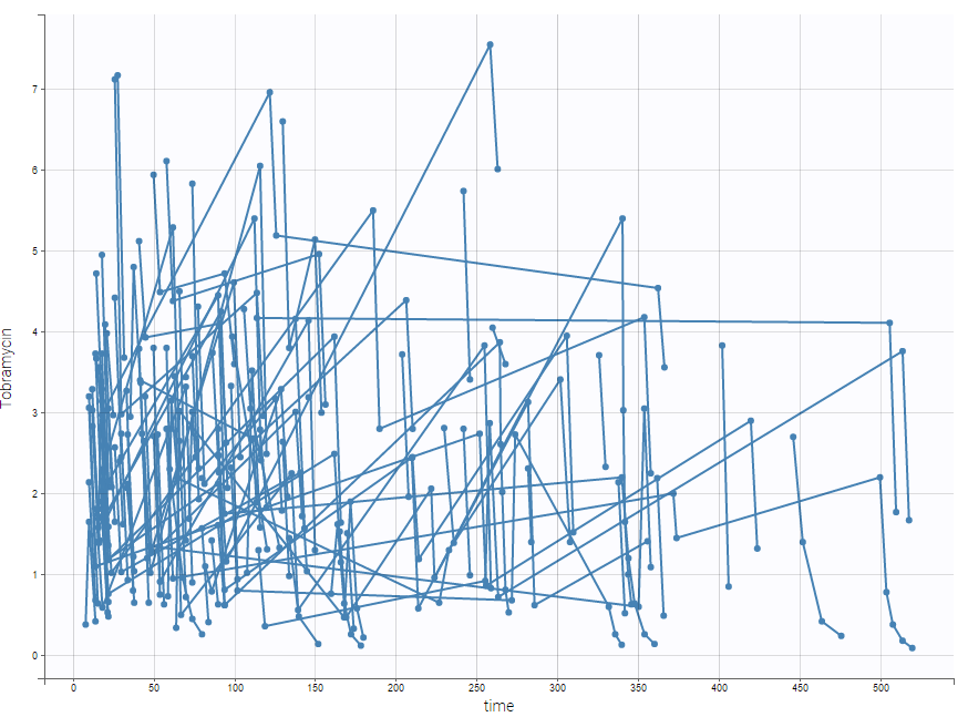
Below is an extract of the data set:
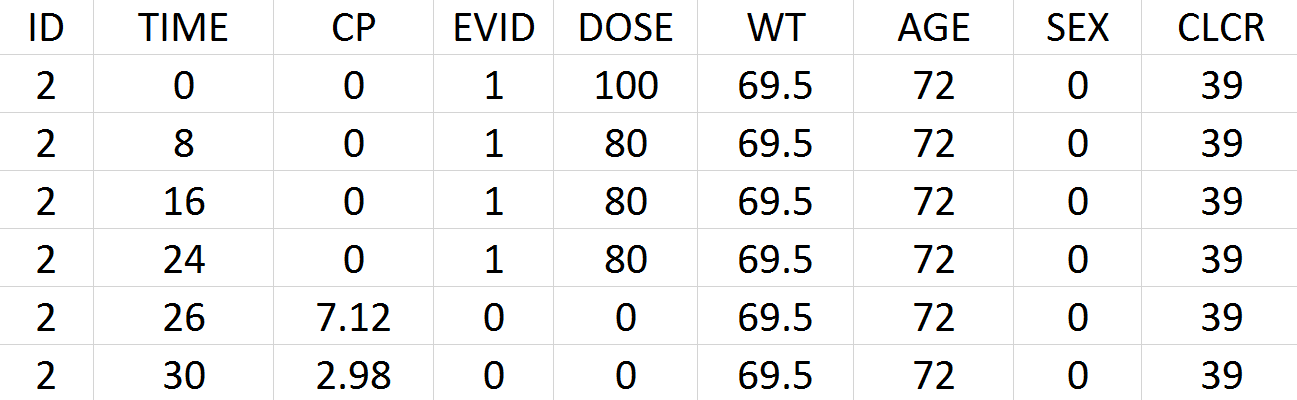
The columns have the following meaning:
- ID: the subject’s ID, column-type ID.
- TIME: the time of the record (administration or measurement) in hours, column-type TIME.
- CP: the measured drug’s concentration in mg/L, column-type OBSERVATION.
- EVID: event identifier, 1 for doses and 0 for response lines (measurements), column-type EVENT ID.
- DOSE: the amount of drug administrated to this subject in mg, column-type AMOUNT.
- WT: weight of the subject in kg, column-type CONTINUOUS COVARIATE.
- SEX: sex of the subject, column-type CATEGORICAL COVARIATE.
- CLCR: creatinine clearance of the subject in mL/min, column-type CONTINUOUS COVARIATE.
Several points can be noticed:
- The four first lines correspond to doses, while the other ones are measurements, as indicated by the EVID column. The MDV column is not necessary. The zeros of the DOSE and CP columns could have been replaced by dots ‘.’ .
- The covariates columns (WT, SEX and CLCR) are filled with the same value for each individual. Covariates must be constant within subjects (or subject-occasions when occasions are defined).
The data set and datxplore project file are in Datxplore demos.
3.1.3.HIV data set
HIV data set
In the COPHAR II-ANRS 134 trial, an open prospective non-randomized interventional study, 115 HIV-infected patients adults started an antiviral therapy. 48 patients were treated with indinavir (and ritonavir as a booster) (treatment A), 38 with lopinavir (and ritonavir as a booster) (treatment B), and 35 with nelfinavir (Treatment C). patients were followed one year after treatment initialization.
Viral load and CD4 cell count were measured at screenin, at inclusion and at weeks 2 (or 4), 8, 16, 24, 36, and 48. Plasma HIV-1-RNA were measured by Roche monitored with a limit of quantification of 50 copies/ml. The results of this trial are reported in Duval and al. (2009). The simulated data set is in Datxplore demos.
On the two following figures, one could see the two outputs with respect to time for all subjects split by treatments. The red circle corresponds to censored data.
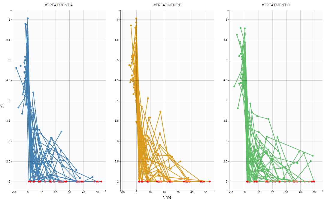

Notice, that these figures were generated using Datxplore.
Simplified HIV data set
The data set for subject 2 can be defined as follows
ID TIME    Y_NCENS Y   CENS    YTYPE   TREATMENT
2   -2.43   4.9443  4.9443  0   1    A
2   -2.43   249 249 0   2    A
2   0   4.5245  4.5245  0   1    A
2   2   2.3546  2.3546  0   1    A
2   2   266 266 0   2    A
2   4.29    268 268 0   2    A
2   8   2.5585  2.5585  0   1    A
2   8   34  34  0   2    A
2   16  352 352 0   2    A
2   24  1.7981  2   1   1    A
2   24  385 385 0   2    A
2   32  348 348 0   2    A
2   43  415 415 0   2    A
Interpretation
One can see the following columns
- ID: the subject ID, column-type ID.
- TIME: the time of the measurement, column-type TIME.
- Y_NCENS: Non censored measurement. Ignored in the representation.
- Y: Considered measurement taking the censoring constraints into account, column-type OBSERVATION.
- CENS: Explicit if the data is censored or not, and the associated type of censoring, column-type CENSORING.
- YTYPE: the type of measurement. In this study, one has two measurements, column-type OBSERVATION ID.
- TREATMENT: Type of treatment, considered as a categorical covariate in our case, column-type CATEGORICAL COVARIATE.
Several points can be noticed.
- There are no dose in the data set.
- There is only a categorical covariate defining the treatment.
- In the presented case, one does not necessary have both measurements at the same time. Indeed, this is not required for data export using Datxplore, nor parameter estimation using Monolix. Moreover, measurements for negative time is possible.
3.1.4.Veralipride data set
This data set has been originally published in:
Veralipride is a benzamide neuroleptic medicine indicated in the treatment of vasomotor symptoms associated with the menopause.
In this dataset, 100 mg doses of veralipride were given to 12 healthy volunteers by oral solution. Individual plasma concentrations of veralipride (ng/ml) were observed at 16 time points during 24h (time is measured in h) after the administration. Doses were given in the morning after an overnight fast, and subjects fasted up to 4 hr after drug administration in each case.
This data set is displayed on the figure below. For some individuals, as the one highlighted on the figure, a double peak in plasma concentrations was observed after oral administration of the solution.
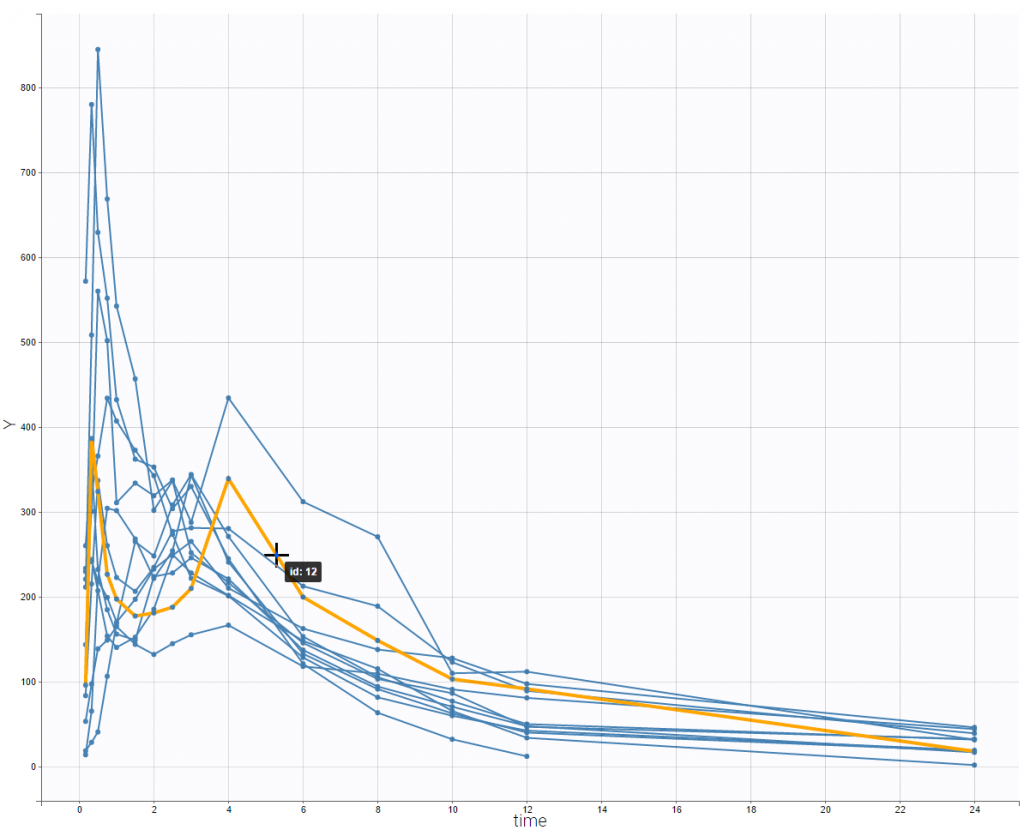
This double peak phenomenon is not systematically noticeable, as can be seen on the next figure.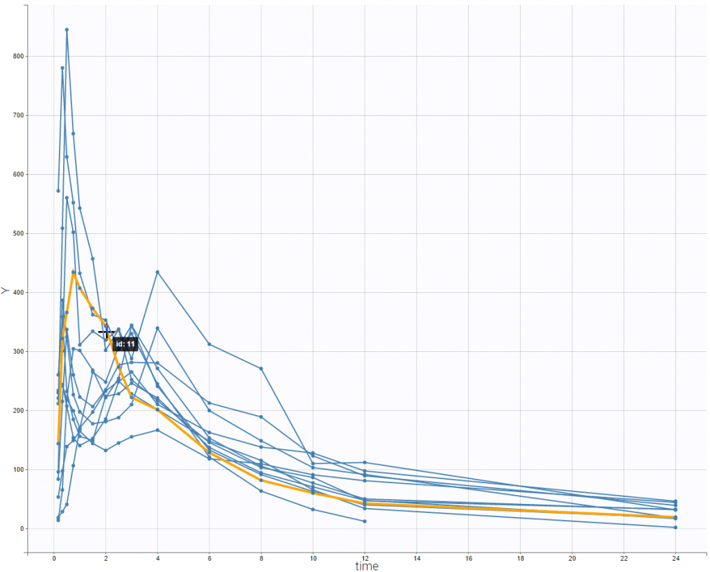
Below is an extract of the data set file:
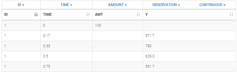
The columns are:
- ID: the subject ID, column-type ID.
- TIME: the time of the measurement or of the dose, column-type TIME.
- AMT: the amount of drug provided to this subject, column-type AMOUNT
- Y: the measurement, column-type OBSERVATION.
The data set and datxplore project file can be in Datxplore demos.
3.1.5.Remifentanil data set
This data set has been originally published in:
Remifentanil is an opioid analgesic drug with a rapid onset and rapid recovery time. It is used for sedation as well as combined with other medications for use in general anesthesia. It is given in adults via continuous IV infusion.
65 healthy adults have received remifentanil IV infusion at a constant diffusion rate between 1 and 8 µg.kg-1.min-1 for 4 to 20 minutes. The data set contains remifentanil admission characteristics (time and rate of infusion), dense measurements of remifentanil blood concentration during infusion and after (PK data), as well as dense electroencephalogram measurements (PD data) recording the depth of anesthesia. In addition, a list of covariates is available: age, gender, and lean body mass (LBM). Moreover, a variable TINFCAT classifies the patients in several categories with similar infusion time.
One can see on the following figure the remifentanil concentrations over time split in two groups (female and male). On each figure, the subjects with age lower than 50 are in blue while the ones with an age over 50 are in green.

On the following figure, one can see the electroencephalogram measurements with respect to time for all subjects.

Below is an extract of the data set file:
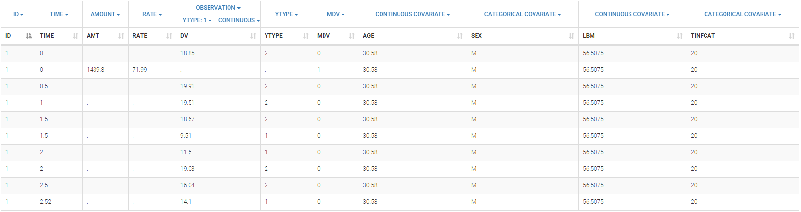
The columns have the following meaning:
- ID: the subject’s ID, column-type ID.
- TIME: the time of the record (administration or measurement) in minutes, column-type TIME.
- AMT: the amount of drug,column-type AMOUT.
- RATE: the rate of drug delivery, column-type INFUSTION RATE.
- DV: remifentanil concentration measurement or electroencephalogram measurement, column-type OBSERVATION.
- YTYPE: the type of measurement. There are two measurement types in this data set: the remifentanil concentration measurement (corresponding to the PK dynamics), and the electroencephalogram measurement (corresponding to the PD-part), column-type OBSERAVTION ID.
- MDV: Missing Data Variable, column-type MDV.
- AGE: Age of the subject in year, column-type CONTINUOUS COVARIATE.
- SEX: sex of the subject (F for female and M for male), column-type CATEGORICAL COVARIATE.
- LBM: lean body mass, column-type CONTINUOUS COVARIATE.
- TINFCAT: Categories of infusion time, column-type CATEGORICAL COVARIATE.
The data set and datxplore project file can be found in Datxplore demos.
3.2.Data sets with discrete count outputs
3.2.1.Epilepsy attacks data set
This data set has been originally published in:
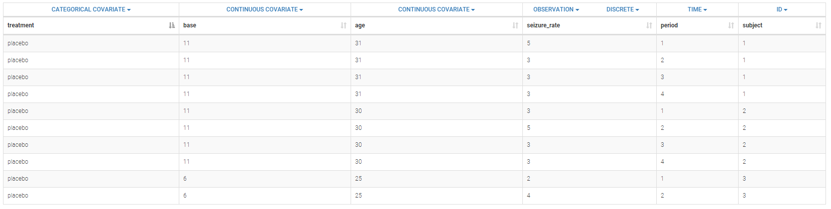
The data arose from a clinical trial of 59 epileptics who were randomized to receive either the anti-epileptic drug progabide or a placebo, as an adjuvant to standard chemotherapy. The hope was that progabide would help to reduce the number of seizures experienced by patients. Patients attended four successive post-randomisation clinic visits, where the number of seizures that occurred over the previous 2 weeks was reported. At baseline, information on the age of the patient and the 8-week pre-randomisation seizure count was recorded.
Below is an extract of the data set:
 The columns have the following meaning:
- treatment: factor with levels placebo progabide indicating whether the anti-epilepsy drug Progabide has been applied or not, column-type CATEGORICAL COVARIATE.
- base: number of epileptic attacks recorded during 8 week period prior to randomization, column-type CONTINUOUS COVARIATE.
- age: age of the patients, column-type CONTINUOUS COVARIATE.
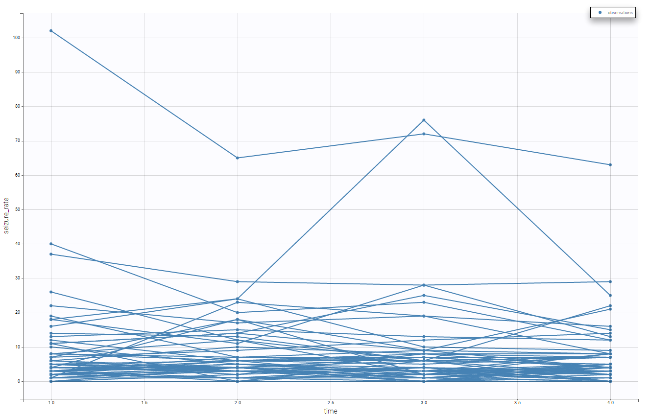
- seizure_rate: number of epilepsy attacks patients have during the follow-up period, column-type OBSERVATION.
- period: measurement period, column-type TIME.
- subject: patient identification number, column-type ID.
Several points can be noticed:
- There are several seizure counts for each individual, thus the time allows to define to which period it is related.
- ID and TIME column are mandatory. Thus, if there is only one count measurement by individual, an additional column with TIME should be added (full of 0 for example).
- The covariates columns (treatment, base and age) are filled with the same value for each individual. Covariates must be constant within subjects (or subject-occasions when occasions are defined).
Moreover, we can split by the covariate treatment and thus see the impact of the treatment
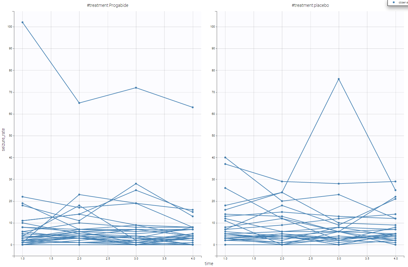
It seems the the subjects with the treatment have lower seizure rate. We can also display it grouped and not in a spaghetti display as in the following

Using that, we have a better understanding of the seizure_rate, and it seems that the treatment is effective.
3.2.2.Crohn's Disease Adverse Events data set
Data set issued from a study of the adverse events of a drug on 117 patients affected by Crohn’s disease (a chronic inflammatory disease of the intestines). In addition to the response variable AE (number of adverse events), 7 explanatory variables were recorded for each patient: BMI (body mass index), HEIGHT, COUNTRY (one of the two countries where the patient lives), SEX, AGE, WEIGHT, and TREAT (the drug taken by the patient in factor form: placebo, d1, d2).
Below is an extract of the data set: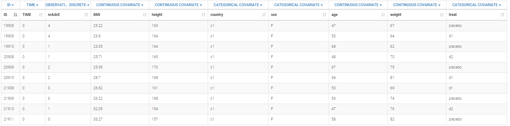
The definition of the columns is the following:
- ID: subject identifier, column-type ID
- TIME: constant to 0, column-type TIME. This column is mandatory. Thus all the values are fixed to 0 as there is only one evaluation.
- nrAdvE: the number of adverse events during the period, column-type OBSERVATION.
- BMI: body mass index, column-type CONTINUOUS COVARIATE
- height: height of the subject in cm, column-type CONTINUOUS COVARIATE
- country: country of the subject, column-type CATEGORICAL COVARIATE
- sex: sex of the subject (M or F), column-type CATEGORICAL COVARIATE
- age: age of the subject (in year), column-type CONTINUOUS COVARIATE
- weight: weight of the subject in kg, column-type CONTINUOUS COVARIATE
- treat: type of treatment, placebo, d1, or d2, column-type CATEGORICAL COVARIATE
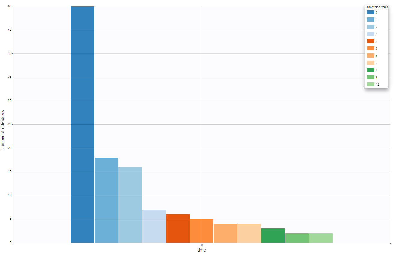
We can see on the following figure the number of adverse events on that period providing a global evaluation of the number of adverse events over the population.
One can split by the categorical covariate treat and see if this covariate as an impact on the number of adverse events. As we can see on the following figure, the drugs seem efficient has we notice that the number of adverse event decrease when drug is used.
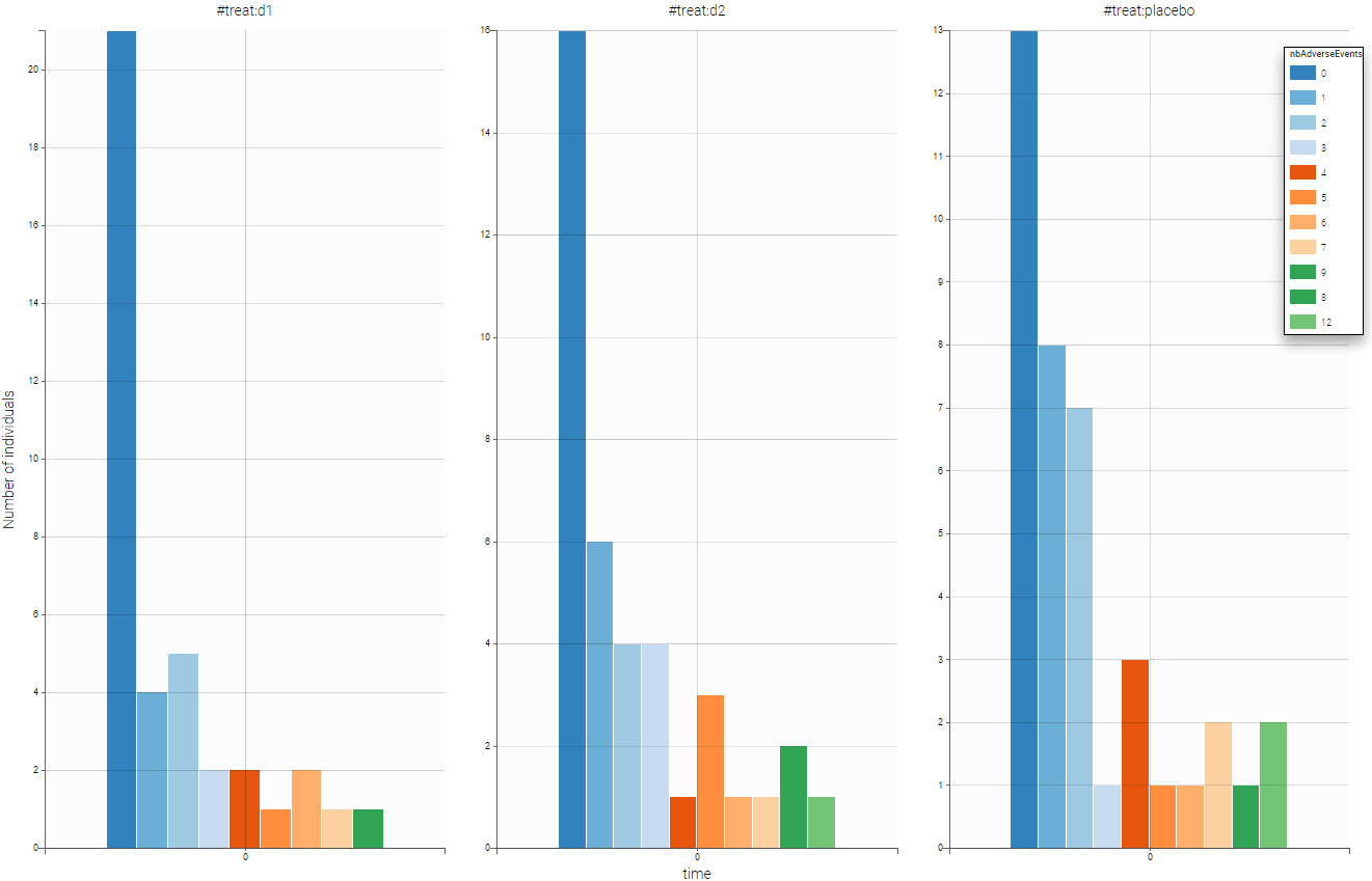
One can also stratify by the other covariate to have a first idea of the dependencies before the statistical population analysis using Monolix.
3.3.Data sets with discrete categorical outputs
3.3.1.Respiratory status data set
In this data set, 111 patients have been administrated a placebo or an active treatment. At randomization and at four visits during the treatment, their respiratory status was determined as being “poor” or “good”, which constitutes the categorical output. Covariates such as center, sex and age were also recorded. The goal was to evaluate the effect of the treatment on the respiratory status.
This data set has been originally published in:
Below we show a snapshot of the data set:
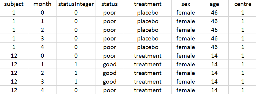
In MonolixSuite, the output categories must be coded as integers. Thus, we have created the column statusInteger where the respiratory status is coded as 0 for “poor” and 1 for “good”. For individual 1 on placebo, the respiratory status is poor at randomization and remains so during the 4 months. For individual 12 on treatment, the respiratory status is poor at randomization and improves to good during the first three months before deteriorating again to poor at month 4.
The definition of the columns is the following:
- subject: patient identifier, column-type ID.
- month: month after treatment start, column-type TIME
- statusInteger: respiratory status coded as integer, 0 for “poor” and 1 for “good”, column-type OBSERVATION.
- status: respiratory status coded as strings “poor” and “good”, column to be ignored
- treatment: type of treatment, active or placebo, column-type CATEGORICAL COVARIATE.
- sex: sex of the patient, female or name, column-type CATEGORICAL COVARIATE.
- age: age of the patient (in years), column-type CONTINUOUS COVARIATE.
- centre: index of the study center, 1 or 2, column-type CATEGORICAL COVARIATE.
The representation of statusInteger with respect to time is proposed on the following figure

Several points can be noticed:
- The categories must be coded as integers.
- There are respiratory status measures for each individual, the month column allows to define at which time the measures were done.
- ID and TIME column are mandatory. Thus, even when there is only one measurement per individual, an additional column with TIME should be added (full of 0 for example).
- Covariates must be constant within subjects (or subject-occasions when occasions are defined).
- In this example, two categories are present (“good” and “poor”), but any number of categories is possible.
When loading this data set into Datxplore, one can easily visualize the number of individuals with “poor” (coded as 0, in dark blue) or “good” (coded as 1, in light blue) respiratory status over time in the case of placebo (left) or active treatment (right):
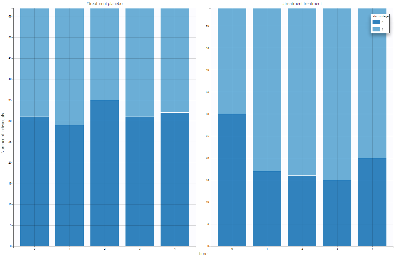
Based on this figure, it seems that the treatment is efficient a priori. We can additionally look at the other covariates and the impact on the output. One can split by sex as can be seen on the following figure.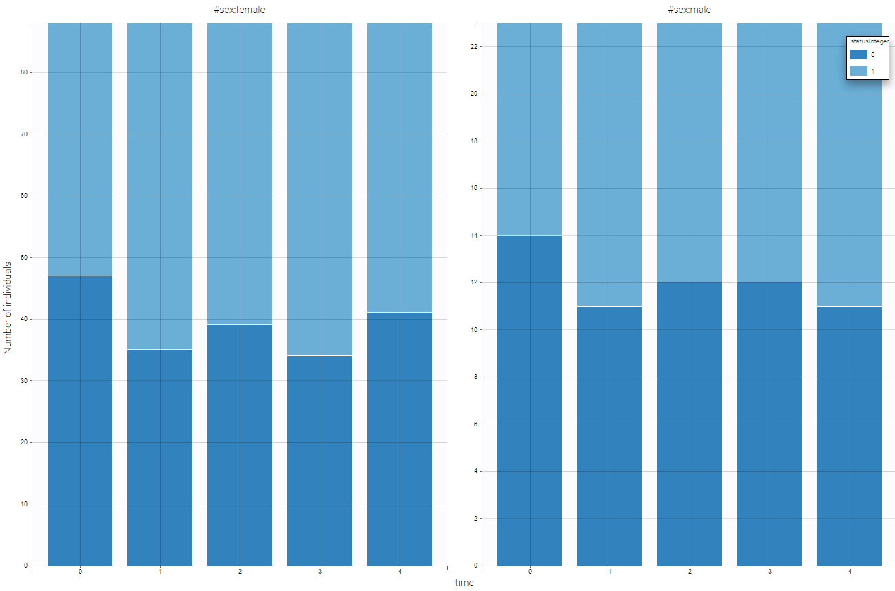
In that case, the sex covariate seems not to influence a lot the output.
3.3.2.Inpatient multidimensional psychiatric data set
This data set has been originally published in:
Hedeker D. and Gibbons R.D. (1996) A computer program for mixed-effects ordinal regression analysis. Computer Methods and Programs in Biomedicine 49, 157-176.
These data are from the National Institute of Mental Health Schizophrenia Collaborative Study and are available here. Patients were randomized to receive one of four medications, either placebo or one of three different anti-psychotic drugs. The protocol indicated subjects were to then be evaluated at weeks 0, 1, 3, 6 to assess severity of illness; additionally some measurements were made at weeks 2, 4, and 5. The primary outcome is item 79 on the Inpatient Multidimensional Psychiatric.
Scale which indicates severity of illness. We will analyze imps79o which is an ordinally scaled version of the original variable imps79 which has the following interpretation
| IMPS | IMPSo |
|---|---|
| 1 and 2 | 1 (not ill or borderline) |
| 3 and 4 | 2 (not ill or borderline) |
| 5 | 3 (markedly) |
| 6 and 7 | 4 (severely or most extremely ill) |
Predictor variables of interest are TxDrug a dummy coded variable indicating treatment with drug or placebo. Below is an extract of the data set:
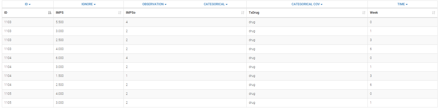 The columns have the following meaning:
- ID: patient identification number, column-type ID
- IMPS: original variable imps79. This column is ignored as we use an ordinally scaled version of this variable.
- IMPSo: ordinally version of imps79, column-type OBSERVATION.
- TxDrug indicates if there is a treatment or the placebo, column-type CATEGORICAL COVARIATE.
- Week: measurement period, column-type TIME.
One can see on the following figure the evolution of the IMPSo with respect to time on both treated patients and patients with placebo.
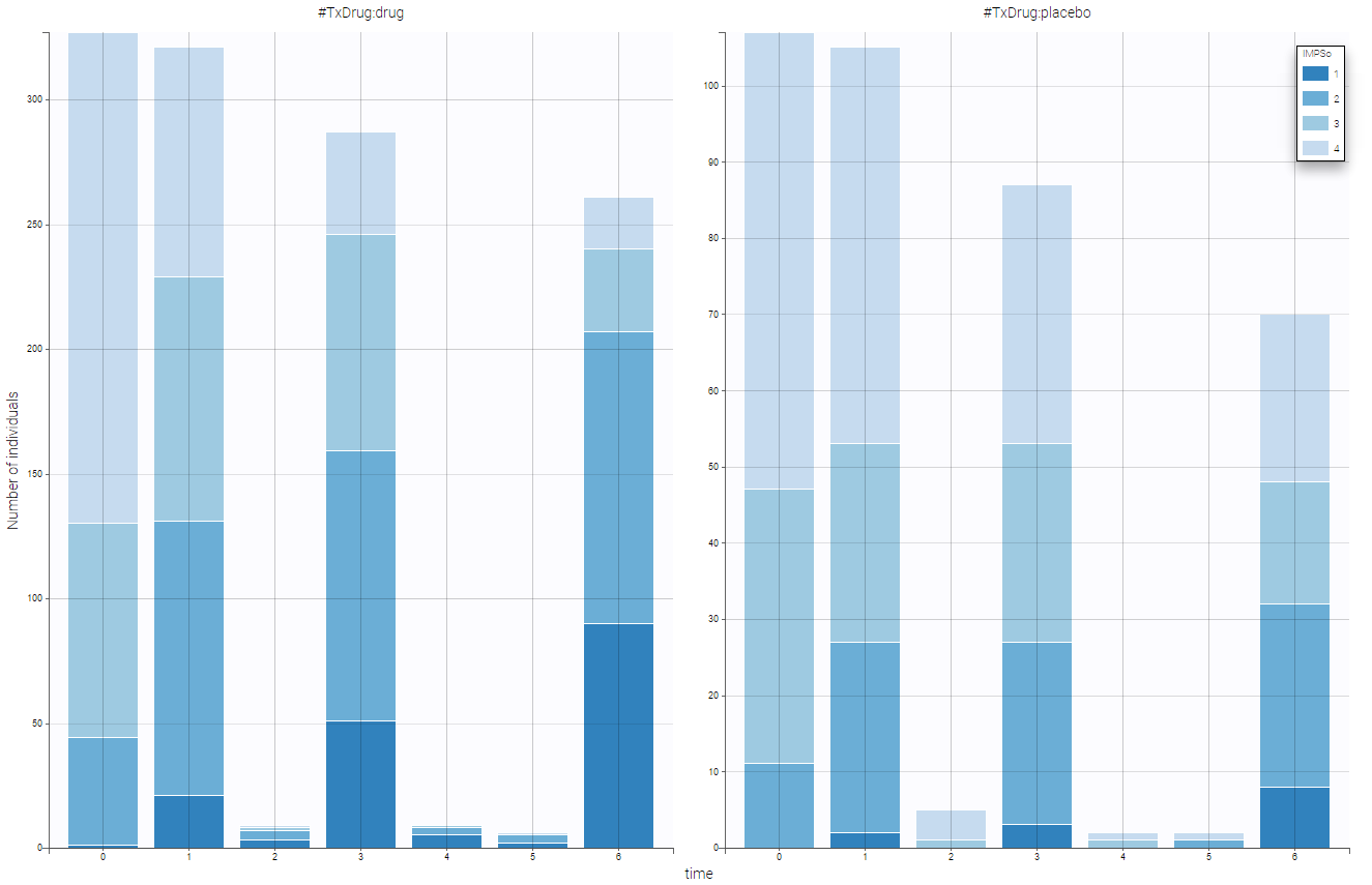
3.3.3.Zylkene data set
This data set has been originally published in:
The putative effects of a tryptic bovine αs1-casein hydrolysate on anxious disorders in cats was investigated. This product is known as alpha-casozepine and patented under the name of Zylkene (Ingredia, Arras, France). Within veterinary practices, 34 cats were recruited by certified behaviorist surgeons. This 56-day trial against placebo showed the statistically positive effect of this product in the management of anxious disorders such as social phobias in cats. Global score, as well as different items (fear of strangers, contact with familiars, general fears, fear-related aggressions, autonomic disorders), were all significantly improved by the use of this natural decapeptide.
Below we show a snapshot of the data set:
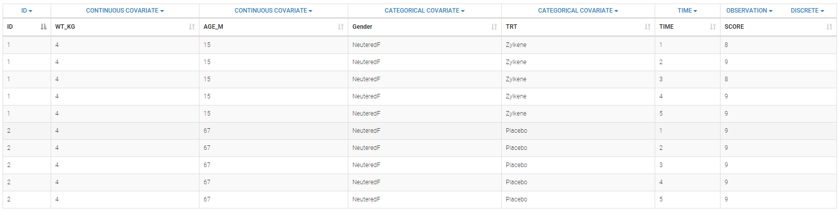
Note that in the MonolixSuite the output categories must be coded as integers. In that cases, observation is a score between 1 and 25. The definition of the columns is the following:
- ID: cat identifier, column-type ID.
- WT_KG: weight of the cat (in kg), column-type CONTINUOUS COVARIATE.
- AGE_M: age of the cat (in month), column-type CONTINUOUS COVARIATE.
- Gender: gender of the cat, Neutered F, Neutered M, or F, column-type CATEGORICAL COVARIATE.
- TRT: type of treatment, Zylkene or placebo, column-type CATEGORICAL COVARIATE.
- TIME: time of the score evaluation, column-type TIME.
- SCORE: global score of emotional state, column-type OBSERVATION.
We can see on the following figure the evolution of all SCORE with respect to time. We see that, when the time increases, the number of cats with a higher score increases too.
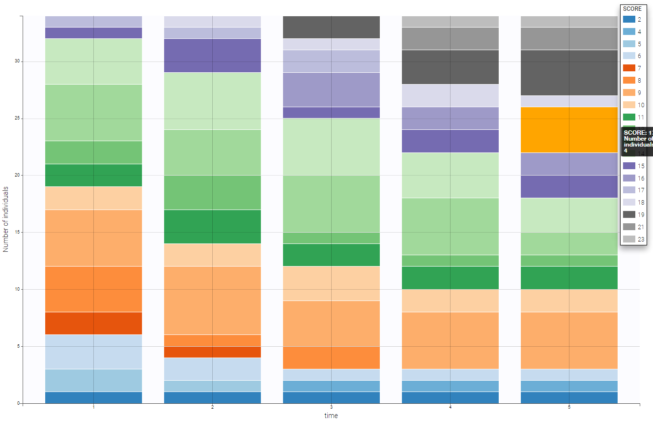
To see the impact of the treatment, we can split by the covariate TRT and see what is the difference between the two groups as on the following figure (placebo on the left and treatment on the right). We see that the treatment seems efficient as the SCORE is better with the treatment
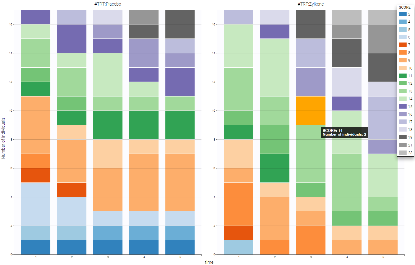
We can do the same with the GENDER categorical covariate, we can create two groups the female (associating F and NeuteredF) and the male (NeutredM). On the contrary to the treatment, the GENDER does not seem to impact the SCORE.
3.4.Event outputs data set
3.4.1.PBC data set
Primary Biliary Cirrhosis is a rare but fatal chronic liver disease of unknown cause, with a prevalence of about 50-cases-per-million population. The primary pathologic event appears to be the destruction of interlobular bile ducts, which may be mediated by immunologic mechanisms.
Between January, 1974 and May, 1984, the Mayo Clinic conducted a double-blinded randomized trial in primary biliary cirrhosis of the liver (PBC), comparing the drug D-penicillamine (DPCA) with a placebo. There were 424 patients who met the eligibility criteria seen at the Clinic while the trial was open for patient registration. Both the treating physician and the patient agreed to participate in the randomized trial in 312 of the 424 cases. The date of randomization and a large number of clinical, biochemical, serologic, and histologic parameters were recorded for each of the 312 clinical trial patients. The data from the trial were analyzed in 1986 for presentation in the clinical literature. For that analysis, disease and survival status as of July, 1986, were recorded for as many patients as possible. By that date, 125 of the 312 patients had died, with only 11 not attributable to PBC. Eight patients had been lost to follow up, and 19 had undergone liver transplantation.
The considered data set comes from Counting Processes and Survival Analysis by T. Fleming & D. Harrington, (1991), published by John Wiley & Sons. On the following figure, one could see the survival curve and the mean number of events with respect to time. Notice, that this figure was generated using Datxplore.
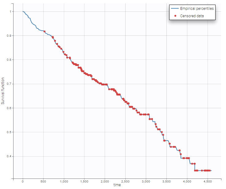 In this data set, there are a lot of available covariates
id       = case number
futime   = number of days between registration and the earlier of death,
           transplantion, or study analysis time in July, 1986
status   = 0=alive, 1=liver transplant, 2=dead
drug     = 1= D-penicillamine, 2=placebo
age      = age in days
sex      = 0=male, 1=female
ascites  = presence of ascites: 0=no 1=yes
hepato   = presence of hepatomegaly 0=no 1=yes
spiders  = presence of spiders 0=no 1=yes
edema    = presence of edema 0=no edema and no diuretic therapy for edema;
          .5 = edema present without diuretics, or edema resolved by diuretics;
           1 = edema despite diuretic therapy
bili     = serum bilirubin in mg/dl
chol     = serum cholesterol in mg/dl
albumin  = albumin in gm/dl
copper   = urine copper in ug/day
alk_phos = alkaline phosphatase in U/liter
sgot     = SGOT in U/ml
trig     = triglicerides in mg/dl
platelet = platelets per cubic ml/1000
protime  = prothrombin time in seconds
stage    = histologic stage of disease
On the two following figure, one could see the survival curve with respect to the treatment. Notice, that this figure was generated using Datxplore.
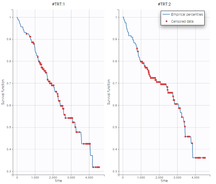
Simplified data set
The data set for subjects 1 and 2 can be defined as follows
ID;TIME;Y;TRT;AGE;SEX;
1;0;0;1;58.7652;1;
1;400;1;1;58.7652;1;
2;0;0;1;56.4463;1;
2;4500;0;1;56.4463;1;
One must indicated the start time of the observation period with Y=0 (at line 1 and 3 for subject 1 and 2 respectively), and the time of event (Y=1) or the time of the end of the observation period if no event has occurred (Y=0). In this simplified data set, subject one had an event at time 400 leading to a line in the data set where Y=1. On the contrary, no event occurred for subject 2. Thus, at the end of the observation (TIME=4500), Y is set to 0.
3.4.2.Oropharynx data set
Oropharynx data set
The following data set provides the data for a part of a large clinical trial carried out by the Radiation Therapy Oncology Group in the United States. The full study included patients with squamous carcinoma of 15 sites in the mouth and throat, with 16 participating institutions, though only data on three sites in the oropharynx reported by the six largest institutions are considered here. Patients entering the study were randomly assigned to one of two treatment groups, radiation therapy alone or radiation therapy together with a chemotherapeutic agent. One objective of the study was to compare the two treatment policies with respect to patient survival. Approximately 30% of the survival times are censored owing primarily to patients surviving to the time of analysis. Some patients were lost to follow-up because the patient moved or transferred to an institution not participating in the study, though these cases were relatively rare.
The considered data set comes from The Statistical Analysis of Failure Time Data, by JD Kalbfleisch & RL Prentice, (1980), Published by John Wiley & Sons.The data set can be seen here, and the corresponding Datxplore project here (notice that both file should be in the same folder to be correctly linked).
On the following figure, one could see the survival curve and the mean number of events with respect to time. Notice, that this figure was generated using Datxplore.
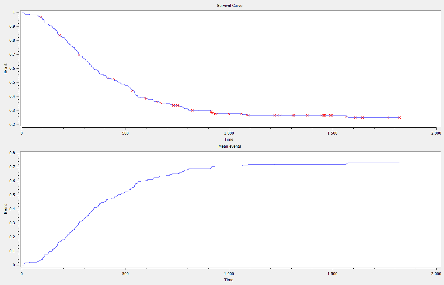
This study included measurements of many covariates which would be expected to relate to survival experience. Six such variables are given in the data (sex, T staging, N staging, age, general condition, and grade). The site of the primary tumor and possible differences between participating institutions require consideration as well.
CASE          Case Number
INST          Participating Institution
SEX           1=male, 2=female
TX        Treatment: 1=standard, 2=test
GRADE         1=well differentiated, 2=moderately differentiated,
              3=poorly differentiated,  9=missing
AGE           In years at time of diagnosis
COND          Condition: 1=no disability, 2=restricted work, 3=requires assistance
              with self care, 4=bed confined,  9=missing
SITE          1=faucial arch, 2=tonsillar fossa, 3=posterior pillar,
              4=pharyngeal tongue, 5=posterior wall
T_STAGE       1=primary tumor measuring 2 cm or less in largest diameter,
              2=primary tumor measuring 2 cm to 4 cm in largest diameter with
              minimal infiltration in depth, 3=primary tumor measuring more
              than 4 cm, 4=massive invasive tumor
N_STAGE       0=no clinical evidence of node metastases, 1=single positive
              node 3 cm or less in diameter, not fixed, 2=single positive
              node more than 3 cm in diameter, not fixed, 3=multiple
              positive nodes or fixed positive nodes
ENTRY_DT      Date of study entry: Day of year and year, dddyy
STATUS        0=censored,  1=dead
TIME          Survival time in days from day of diagnosis
On the two following figure, one could see the survival curve and the mean number of events with respect to time for two groups, the first groups concerns the subjects younger than 55 years and the other group concerns the other one. Notice, that this figure was generated using Datxplore.
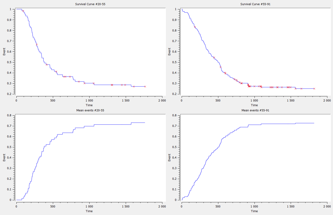
Simplified Oropharynx data set
The data set for subjects 47 and 48 can be defined as follows
ID;INST;SEX;TRT;GRADE;AGE;COND;SITE;T_STAGE;N_STAGE;ENTRY_DT;Y;Time
47;4;1;2;2;49;3;1;4;3;5669;0;0
47;4;1;2;2;49;3;1;4;3;5669;1;74
48;3;1;1;1;44;1;1;3;1;2769;0;0
48;3;1;1;1;44;1;1;3;1;2769;0;1609
One must indicated the start time of the observation period with Y=0 (at line 1 and 3 for subject 47 and 48 respectively), and the time of event (Y=1) or the time of the end of the observation period if no event has occurred (Y=0). In this simplified data set, subject 47 had an event at time 74 leading to a line in the data set where Y=1. On the contrary, no event occurred for subject 48. Thus, at the end of the observation (TIME=1609), Y is set to 0.
3.4.3.Veterans’ Administration Lung Cancer data set
In a study conducted by the US Veterans Administration, male patients with advanced inoperable lung cancer were given either a standard therapy or a test chemotherapy. Time to death was recorded for 137 patients, while 9 left the study before death. Various covariates were also documented for each patient.
The primary goal of the study was to assess if the test chemotherapy is beneficial. Secondary goals included the analysis of covariates as prognostic variables.
This data set has been published in D Kalbfleisch and RL Prentice (1980), The Statistical Analysis of Failure Time Data. Wiley, New York. The data set can be seen in Datxplore demos.
A snapshot of the data set in shown below:
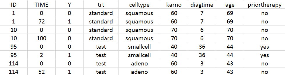
The TIME and Y columns are interpreted in the following way: the observation period for individual 1 start at time 0 and the event occurs at time 72 (i.e 72 days after the enrollment). For individual 10, the start time is also 0 and by the end of the observation period for this individual at time 100, no event has yet occurred.
The structure of the data file is the following:
- ID: ID of the patient, column-type ID
- TIME: time of start of the observation period (if Y=0, first occurrence), death (if Y=1) or censoring (if Y=0, second occurrence), column-type TIME.
- Y: 0 to indicate the start of the observation period or censoring and 1 to indicate death, column-type OBSERVATION.
- trt: treatment type, column-type CATEGORICAL COVARIATE
- celltype: histological type of the tumor, categorical covariate, column-type CATEGORICAL COVARIATE
- karno: Karnofsky performance score that describes the overall patients status at the beginning of the study, column-type CONTINUOUS COVARIATE
- diagtime: Time between diagnosis and start of the study (in month), column-type CONTINUOUS COVARIATE
- age: age of the patient (in years), column-type CONTINUOUS COVARIATE
- priortherapy: indicates if the patient has received another therapy before the current one, column-type CATEGORICAL COVARIATE
Using Datxplore, one can visualize the Kaplan-Meier curve. The censored data are indicated by red points.
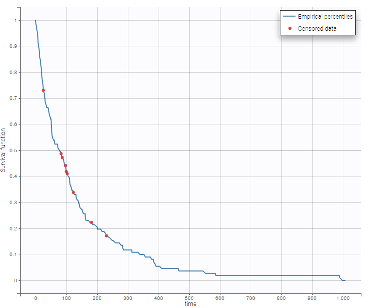
3.4.4.NCCTG lung cancer data set
The North Central Cancer Treatment Group (NCCTG) data set records the survival of patients with advanced lung cancer, together with assessments of the patients performance status measured either by the physician and by the patients themselves. The goal of the study was to determine whether patients self-assessment could provide prognostic information complementary to the physician’s assessment. The data set contains 228 patients, including 63 patients that are right censored (patients that left the study before their death).
This data set has been originally presented and analyzed in Loprinzi et al. (1994). Prospective evaluation of prognostic variables from patient-completed questionnaires. North Central Cancer Treatment Group. Journal of Clinical Oncology : Official Journal of the American Society of Clinical Oncology, 12(3), 601–607. The data set can be downloaded in Datxplore demos.
A snapshot of the data set is displayed below:
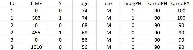
The observation period for individual 1 start at 0 and the death event is observed at time 306. On the opposite, individual 3 left the study at time 1010, before his death.
The meaning of the columns is the following:
- ID: ID of the patient, column-type ID
- TIME: time of start of the observation period (if Y=0, first occurrence), death (if Y=1) or censoring (if Y=0, second occurrence), column-type TIME.
- Y: 0 to indicate the start of the observation period or censoring and 1 to indicate death, column-type OBSERVATION.
- age: age of the patient (years), column-type CONTINUOUS COVARIATE
- sex: sex of the patient (F for female, M for male), column-type CATEGORICAL COVARIATE
- ecogPH: ECOG (Eastern Cooperative Oncology Group) performance status assessed by the physician, on a scale from 0 (fully active) to 5 (dead). For information on the scale, click here, column-type CATEGORICAL COVARIATE
- karnoPH: Karnofsky performance status, assessed by the physician, on a scale from 0 (dead) to 100 (completely healthy). More details about the scale can be found here, column-type CONTINUOUS COVARIATE.
- karnoPAT: Karnofsky performance status, assessed by the patient, column-type CONTINUOUS COVARIATE
Using Datxplore, one can visualize the Kaplan-Meier kurve. The censored data are indicated by red points.
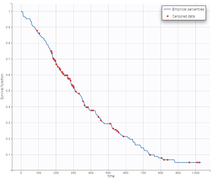
3.4.5.Cardiovascular data set
Data come from the 1991 Arizona cardiovascular patient files. A subset of the fields was selected to model the differential length of stay for patients entering the hospital to receive one of two standard cardiovascular procedures: CABG and PTCA. CABG is the standard acronym for Coronary Artery Bypass Graft, where the flow of blood in a diseased or blocked coronary artery or vein has been grafted to bypass the diseased sections. PTCA, or Percutaneous Transluminal Coronary Angioplasty, is a method of placing a balloon in a blocked coronary artery to open it to blood flow. It is a much less severe method of treatment for those having coronary blockage, with a corresponding reduction in risk.
Below we show a snapshot of the data set:
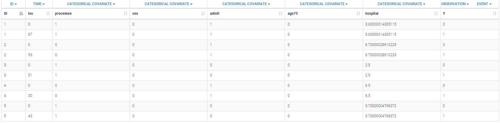
The definition of the columns is the following:
- ID: patient identifier, column-type ID
- los: time in days when the patient goes out of the hospital, column-type TIME
- procedure: procedure used, 1 or 0 (1 for CABG and 0 for PTCA), column-type CATEGORICAL COVARIATE
- sex: sex of the patient, 1 or 0 (1 for Male and 0 for female), column-type CATEGORICAL COVARIATE
- admit: type of admission, 1 or 0 (1 for Urgent/Emergency and 0 for elective), column-type CATEGORICAL COVARIATE
- age75: is the subject’s age over 75 years, column-type CATEGORICAL COVARIATE
- hospital: string describing the hospital, column-type CATEGORICAL COVARIATE
- Y: event type (0 to enter in the hospital, 1 when the event ‘The subject leaves the hospital’ happens), column-type OBSERVATION
The representation of the Keiplan-Meier curve with respect to time is presenter below.
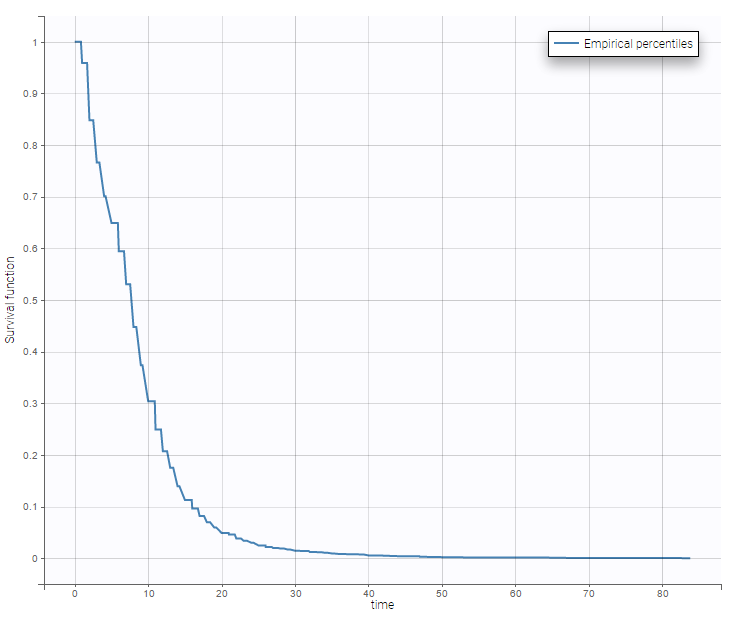
3.5.Joint data sets
3.5.1.Warfarin data set
Warfarin data set
This data set has been originally published in:
Warfarin is an anticoagulant normally used in the prevention of thrombosis and thromboembolism, the formation of blood clots in the blood vessels and their migration elsewhere in the body, respectively. The data set provides set of plasma warfarin concentrations and Prothrombin Complex Response in thirty normal subjects after a single loading dose. A single large loading dose of warfarin sodium, 1.5 mg/kg of body weight, was administered orally to all subjects. Measurements were made each 12 or 24h.
On the two following figure, one could see the concentration and the effect with respect to time for all subjects.

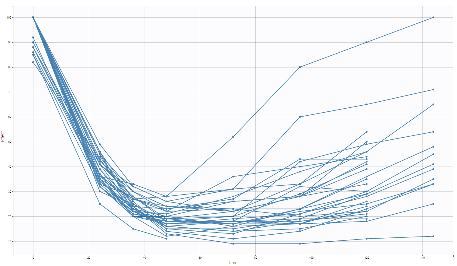
The data set for subject one can be defined as follows
id time    amt dv  dvid    wt  age sex
1   0   100 .   1   66.7    50  1
1   0   .   100 2   66.7    50  1
1   24  .   9.2 1   66.7    50  1
1   24  .   49  2   66.7    50  1
1   36  .   8.5 1   66.7    50  1
1   36  .   32  2   66.7    50  1
1   48  .   6.4 1   66.7    50  1
1   48  .   26  2   66.7    50  1
1   72  .   4.8 1   66.7    50  1
1   72  .   22  2   66.7    50  1
1   96  .   3.1 1   66.7    50  1
1   96  .   28  2   66.7    50  1
1   120 .   2.5 1   66.7    50  1
1   120 .   33  2   66.7    50  1
Interpretation
One can see the following columns
- id: the subject ID, column-type ID
- time: the time of the measurement or of the dose, column-type TIME.
- amt: the amount of drug provided to this subject, column-type AMOUNT.
- dv: the measurement, column-type OBSERVATION.
- dvid: the type of measurement. In this study, one has two measurement, the concentration measurement (corresponding to the PK dynamics), and the Prothrombin Complex Response (corresponding to the PD-part), column-type OBSERVATION ID.
- wt: Weight of the subject, column-type CONTINUOUS COVARIATE.
- age: Age of the subject, column-type CONTINUOUS COVARIATE.
- sex: Sex of the subject, column-type CATEGORICAL COVARIATE.
Several points can be noticed.
- The first line corresponds to a dose, while the other ones are measurements. This explains the dot in the CONC column for the first line and the dots in the AMT column for the other ones.
- The covariates columns (the continuous wt and the categorical covariates age and sex) are filled with the same values. Even though it is not necessary, we encourage the user to fill the columns for readability and usage reasons.
- In the presented case, both PK and PD measurements are at the same time, this is not required for data exploration using Datxplore, nor parameter estimation using Monolix.
- Finally, notice that no initial washout is needed at the beginning as by default, the null initial condition is used for parameter estimation.
Interestingly, one can display the Effect with respect to the Concentration in order to have an idea on how to model the interaction between the PD and the PK part.
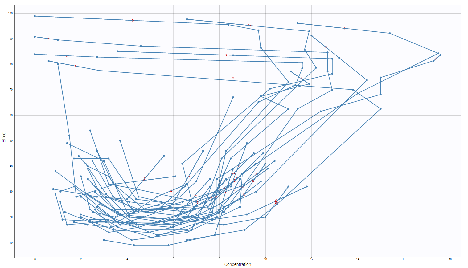
Then, the response does not seem to be direct. Notice that, as the observation times are no the same between the PK and the PD, interpolation is made to propose this kind of plot. One can also focus on one individual in particular as on the following figure
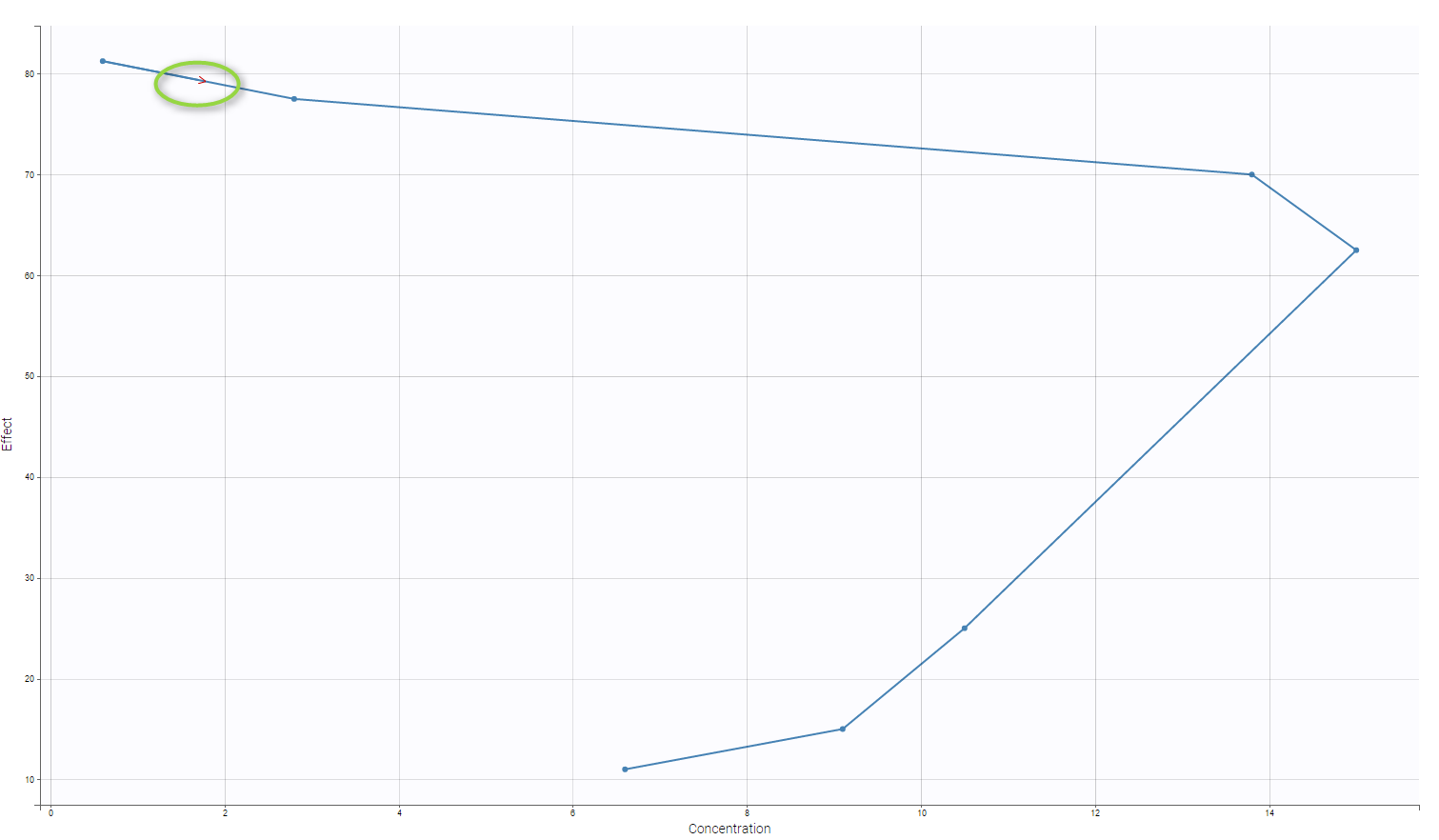
Notice that we also propose a red arrow to describe the evolution of time.
3.5.2.PSA and survival data set
This data set has been originally published in:
It contains PSA kinetics and survival data for 400 men with metastatic Castration-Resistant Prostate Cancer (mCRPC) treated with docetaxel and prednisone, the first-line reference chemotherapy, which constituted the control arm of a phase 3 clinical trial. In this context of advanced disease, the incidence of death is high and the PSA kinetics is closely monitored after treatment initiation to rapidly detect a breakthrough in PSA and propose rescue strategies. In more details:
- PSA kinetics: 6627 PSA measurements were collected, among which roughly 20% were pretreatment, 60% on treatment, and 20%posttreatment. 2.5% are below the limit of quantification (LoQ),set at 0.1 ng.ml−1.
- survival: 286 patients deceased (71.5%), leading to a median survival of 656 days.
PSA measurements are displayed on the figure below. Since the data density is too high to see clearly, the next figure is a selection of six individuals, that allows to identify the shape of PSA measurements followed by most individuals: a decrease of PSA concentration after the treatment initiation at time zero, followed by an increase some time later due to resistance.
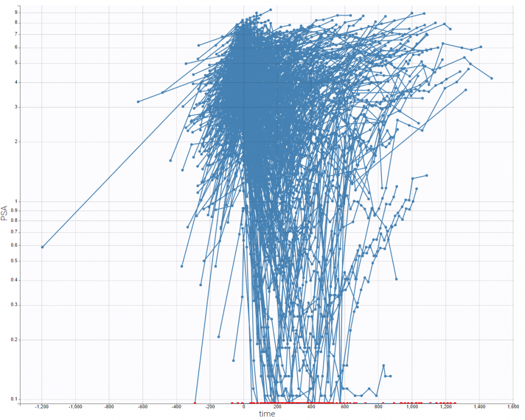
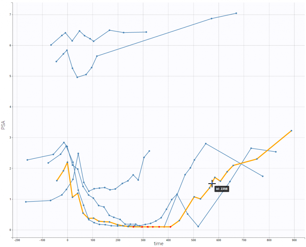
The following figure shows the Kaplan-Meier curves for the survival data split in two groups by the median time of end of treatment
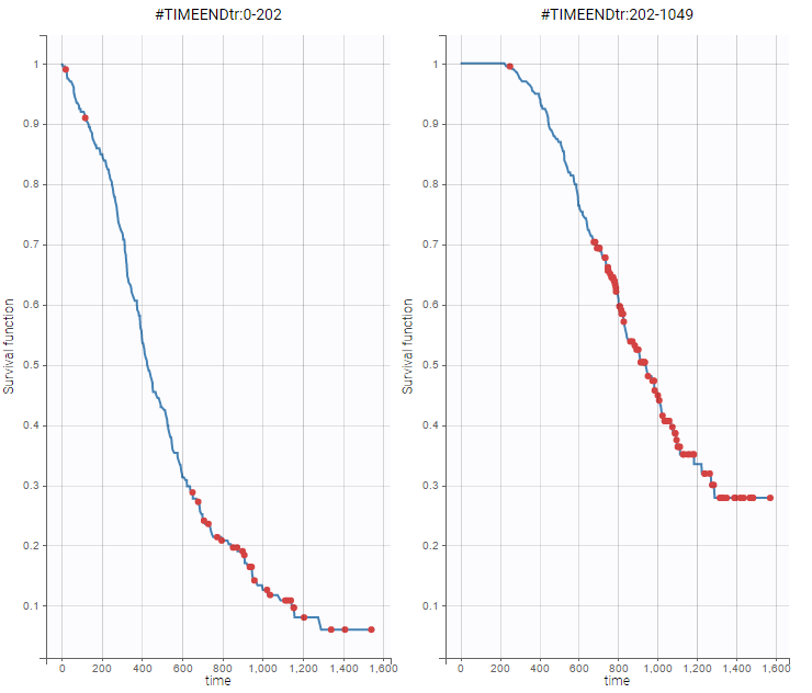
Below is an extract of the data set file:

The columns are:
- TIME: the time of the measurement or of the dose, column-type TIME.
- ID: the subject ID, column-type ID.
- Y: measurements of PSA concentration in ng.ml−1, or death events, column-type OBSERVATION.
- CENS: CENS=1 indicates values below the limit of quantification (LoQ), column-type CENSORING.
- YTYPE: the type of measurement. There are two measurement types in this data set: the PSA concentration measurement (corresponding to the PD), and death events, column-type OBSERVATION ID.
- TIME_ENDtr: day of end of treatment, column-type CONTINUOUS COVARIATE.
4.FAQ
4.1.FAQ
Evolution
- What are the evolution in this version compared to the previous version (2016R1)? All the evolution can be found here.
- Can I get the documentation for the data set associated with the 2016R1 version? Of course, you can download it here.
Questions about format
- Which file formats are supported? Text and comma-separated values file are allowed. The file extension should preferably be .txt or .csv.
- Should I have a header line? Yes, having a header line is mandatory.
- Are there restrictions on header names? No, there is no limitation in terms of names nor on character number. However, some characters are not allowed as in the rest of the data file (see here).
- Which column types are mandatory? The ID, and OBSERVATION column-types are mandatory. All others are optional.
- Which column-types are possible? The complete list of supported column-types can be found here.
- Which separators are allowed? The supported separators are comma (“,”), semicolon (“;”), space (” “), and tab (“\t”).
- Which characters are allowed in strings? The list of allowed characters can be found here.
- What does “.” mean? The “.” can be used in almost all the lines of the data set but has several meaning depending on the context. A summary can be found here.
- How can I ignore some response-lines of my data set? Use IGNORED OBSERVATION=1 for that.
- How can I ignore some dose-lines of my data set? Use EVENT ID=2
- Can I specify time in hour or in days? Yes, all the possible formats are defined here.
- Can the data be split into several files (for instance one file for dosing and one for observations)? No. All the data must be grouped into a single file.
Questions about units
- How are units handled? Units are free but must be consistent. For instance TIME, INFUSION RATE, INFUSION DURATION, INTERDOSE INTERVAL must have the same TIME units. With models from the libraries, no unit conversion is done. Thus, if in the data set TIME is in hours, rate constant parameters will be /hours. If in the data set the AMOUNT is in mmol and the concentration in mM, then the volume parameter will be in L.
- Is it possible to automatically convert units? No.
- Are the units visible in the graphical user interface of Monolix? No.
Questions about format difference with NONMEM
- What are the differences between Monolix and Nonmem in terms of data set? The few differences are listed here.
- What is the equivalent of the NONMEM CMT column? Depending on the usage of the CMT column, it can correspond to the OBSERVATION ID column-type, or the ADMINISTRATION ID column-type. All differences between NONMEM and the MonolixSuite are listed here.
Questions about subjects and occasions
- Must all lines corresponding to the same individual be grouped? No, this is not necessary. All lines with the same ID will be assigned to the same individual, whatever their order or grouping.
- How can I define occasions? For that, you can use the OCCASION column-type as explained here.
Questions about time
- Must the times be in ascending order? For a given individual, the times do not need to be in order. The sorting will be done automatically.
- Can I specify time in hour or in days? Yes, all the possible formats are defined here.
- Can time have negative values? Yes.
- For time-to-event data, do I have to indicate the start time? Yes, it must be explicitly stated, for instance with TIME=0 and OBSERVATION=0. Guidelines for data set formatting for time-to-event data are given here.
Questions about responses and observations
- Are non-continuous data types (such as count, time-to-event and categorical data) supported? Yes. Exemples of data set for non-continuous data types are presented here.
- Which value should I enter in the OBSERVATION column-type for BLQ values? In the OBSERVATION column-type, give the limit of quantification (LOQ). To mark the observations as being BLQ, use the CENSORED column-type. To indicate a censoring interval, use the LIMIT column-type in addition.
- Can my data set contain different types of observations? Yes, use the OBSERVATION ID column to define to which type of data the line corresponds. An example data set with different types of observations is presented here.
- What happen if I define both a dose and a response in the same line? Depending on the values, it can be a dose, a response. To see all the configurations, see here.
Questions about dose regimen
- How are steady-state doses handled? In case of a steady-state dose, 5 additional doses are added before the steady-state dose, in order to reach steady-state. More details can be found here.
- What happen if I define both a dose and a response in the same line? Depending on the values, it can be a dose, a response. To see all the configurations, see here.
- For dose-lines, should I specify the compartment into which the dose is introduced? No. In the MonolixSuite, the matching between the data (dose and observation lines) and the model (administrations and predictions) is done using identifiers, not based on compartment numbers. To assign a dose to a specific administration of the model (oral or iv macros for classical PK models, depot macro for more complex ODEs), the column ADMINISTRATION ID is used. The identifier in the ADMINISTRATION ID column should match the “adm=” field of the macro.
- If I have several outputs, should I duplicate the dosing information? No.
- If a dose is split in two absorption routes, should I duplicate the dosing information? No. The same dose line can be split in different fractions using the bioavaila
Questions about covariates
- Can I have time-varying covariates? Continuous (CONTINUOUS COVARIATE) and categorical (CATEGORICAL COVARIATE) covariates must be contant within a subject-occasion. If a continuous covariate varies with respect to time, the first value in time will be used for the entire subject-occasion. Time-varying continuous covariates can be tagged as regressors (column-type REGRESSOR) to be used as such. Examples are proposed here.
Questions about controls and events
- How can I ignore certain response-lines of my data set? Use IGNORED OBSERVATION=1 for that.
- Are the MDV and EVID columns necessary? These columns are not mandatory and most of the time not necessary.
- How can I define a time at which I which the output the predictions, even if I have no observation? No, use Simulx for simulations.
4.2.Translating your dataset from NONMEM format to the Monolix Suite format
The required format for the data set in NONMEM and in the Monolix Suite is very similar. Usually only few changes (if any) are required to go from one format to the other one.
General formatting
- Column names: in the Monolix Suite column names are not restricted in length, and not restricted to uppercase format. Special characters such as spaces ” “, stars “*”, parentheses or brackets “(“, dashes “-“, slashes “/” are supported but are replaced by “_” in the interface and results.
- Header line: no need to start the header line with the “#” character in the Monolix Suite, the column headers line will be recognized automatically.
- Number of columns: there is no limitation of the number of columns in the Monolix Suite
Dose column-types
- STEADY STATE column: When a data set contains a column with column-type STEADY STATE (formerly SS), there must be a column with column-type INTERDOSE INTERVAL (formerly I)I. If STEADY STATE>0, then the value in the INTERDOSE INTERVAL column must be strictly positive. In case of steady-state, steady-state formulas are not used. Instead, additional doses (5 by default) are added before the STEADY STATE dose to reach steady-state.
- INFUSION RATE and INFUSION DURATION: in case of an infusion, in the Monolix Suite, it is possible to define either the rate (INFUSION RATE column-type, formerly RATE) or the duration (INFUSION DURATION column-type, formerly TINF). The rate and the duration are related to each other via the amount: TINF=RATE/AMT. Negative values in the RATE column-type result in a bolus, when used in combination with the iv macro (and models from the library with iv). When used in combination with the oral macro (and models from the library with oral0 or oral1), the RATE column is ignored if the value is negative and an error is triggered if the value is positive. If infusion duration is defined in the model (parameter or fixed value), the RATE column is not necessary (in opposition to NONMEM, where RATE=-1 and RATE=-2 are used).
- CMT column: in NONMEM, for observation-lines, CMT specifies the compartment from which the predicted value of the observation is obtained. For dose-lines, CMT specifies the compartment into which the dose is introduced. In the MonolixSuite, the matching between the data (dose and observation lines) and the model (administrations and predictions) is done using identifiers, not based on compartment numbers. To assign a dose to a specific administration of the model (oral or iv macros for classical PK models, depot macro for more complex ODEs), the column ADMINISTRATION ID (formerly ADM) is used. The identifier in the ADMINISTRATION ID column should match the “adm=” field of the macro. To assign an observation to a prediction, the column OBSERVATION ID (formerly YTYPE) is used. Observation lines with OBSERVATION ID=1 will be assigned to the first output (output = {…} statement in the model file), lines with OBSERVATION ID=2 to the second output, etc. Note that the default values for the administration id in administration macros or in the pkmodel macro is adm=1. Similarly, in case of a single output, OBSERVATION ID=1 by default (while in NONMEM, the central compartment may have number 1 or 2). In the ADMINISTRATION ID column-type, negative values are not allowed. Turning off compartments should instead be defined in the model file.
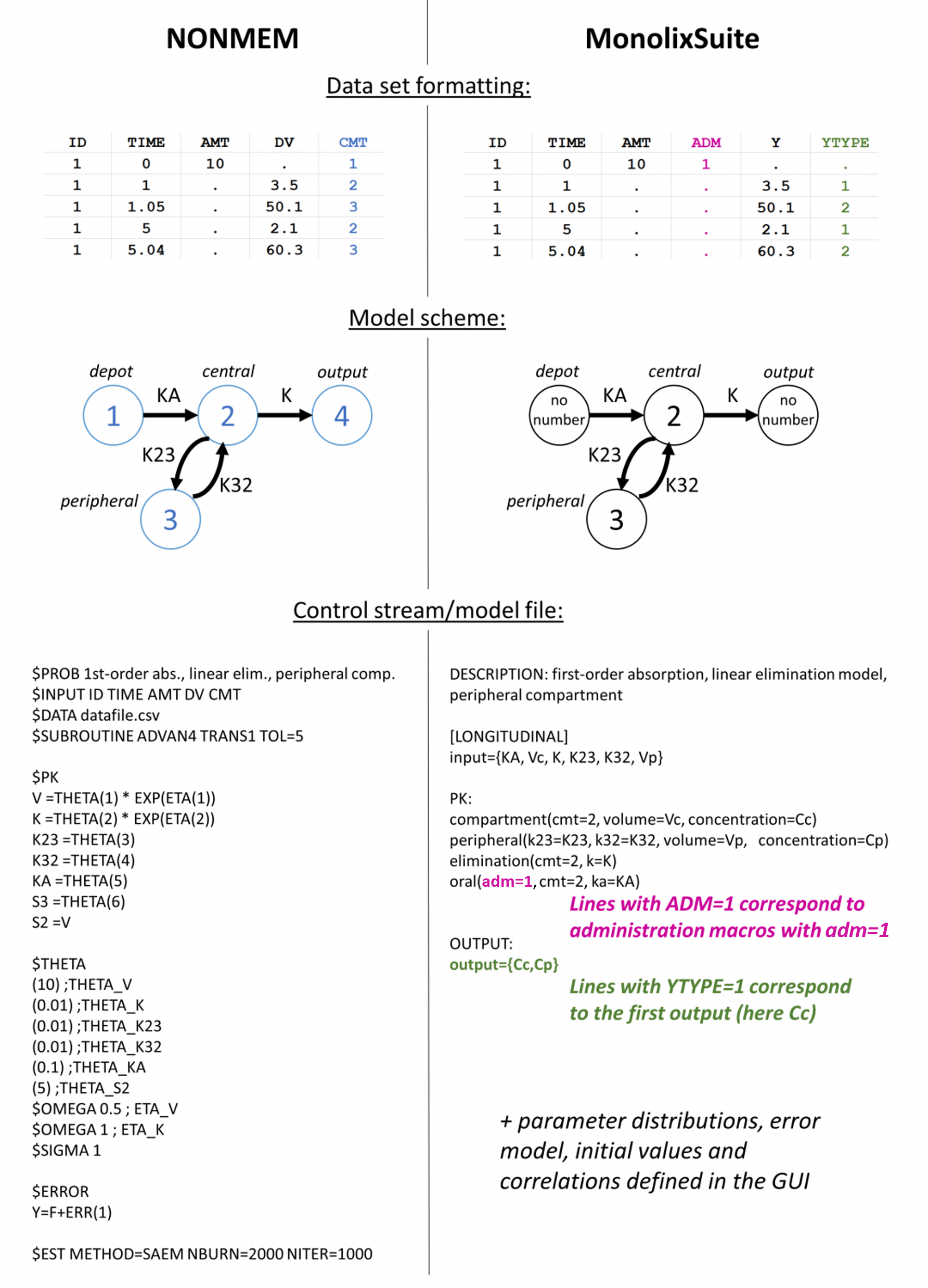
Control and event columns-types
- EVID column-type: in the Monolix Suite, the EVENT ID (formerly EVID) column is not mandatory, since dose-events (EVENT ID=1) and response-events (EVENT ID=0) are automatically recognized. The Monolix Suite also recognizes EVENT ID=2 (“Other event”), EVID=3 (“Reset event”), and EVID=4 (which corresponds to a reset to initial values immediately followed by a dose). EVID=4 creates a new occasion for the individual. In NONMEM, EVID=2 is sometimes used to define a time point at which one would like to predict a concentration, without having an observation. In the Monolix Suite, no prediction will be outputted for that time in the output files.
- MDV column-type: the IGNORED OBSERVATION (MDV) column is not mandatory in the Monolix Suite. Dose-lines and observation-lines will be recognized automatically based on their contents. Yet the IGNORED OBSERVATION column can be useful to force a response-line to be ignored (IGNORED OBSERVATION=1). Several IGNORED OBSERVATION columns are allowed, in this case a synthetic IGNORED OBSERVATION value is computed. In the Monolix Suite, IGNORED OBSERVATION can in addition take the value IGNORED OBSERVATION=2, which is identical to IGNORED OBSERVATION = 1. Note that no prediction will be made at that time point in the output files. Simulx can be used to obtain predictions from a model at different time points.
Response column-types
- Censored data: in the Monolix Suite, censored data should be tagged in the data set using additional columns with CENSORING (formerly CENS) to mark censored observation, and if necessary LIMIT (give other interval boundary) column-types. The LOQ value is indicated in the OBSERVATION column. Censored data are then automatically taken into account in the likelihood in a rigorous statistical way. If only the CENSORING column is used, the method in the MonolisSuite is equivalent to the so-called M3 method. When both CENSORING and LIMIT are used, the method in equivalent to M4.
Subject identification columns-types
- ID column-type: in NONMEM all lines related to a single individual must be in one block, which is not the case in the Monolix Suite. If the ID column contains the following IDs: [1,1,1,2,2,1,1], NONMEM will consider that the dataset comprise three individuals with IDs 1 (with 3 observations), 2 (with 2 observations) and 1_1 (with 2 observations). In the Monolix Suite, two individuals are considered, with IDs 1 (with 5 observations) and 2 (with 2 observations).
Time column-types
- TIME column-type: values in the time column can be negative in the Monolix Suite.
Covariates and regression column-types
- Covariates: in the Monolix Suite, columns corresponding to continuous covariates must be set to the CONTINUOUS COVARIATE (formerly COV) column-type, and categorical covariates to the CATEGORICAL COVARIATE (formerly CAT) column-type.
- Regression variables: in the Monolix Suite, regression variables must be set to the REGRESSOR (formerly X) column-type. If several regression variables are used, their order must be the same in the dataset and in the “input” field of the model file. Interpolation between two regressor values is done using “last observation carried forward” in Monolix, while it is “next observation carried backward” in Nonmem. When converting a Nonmem dataset to Monolix format, the time-varying regressor columns must be shifted one cell up for each individual.
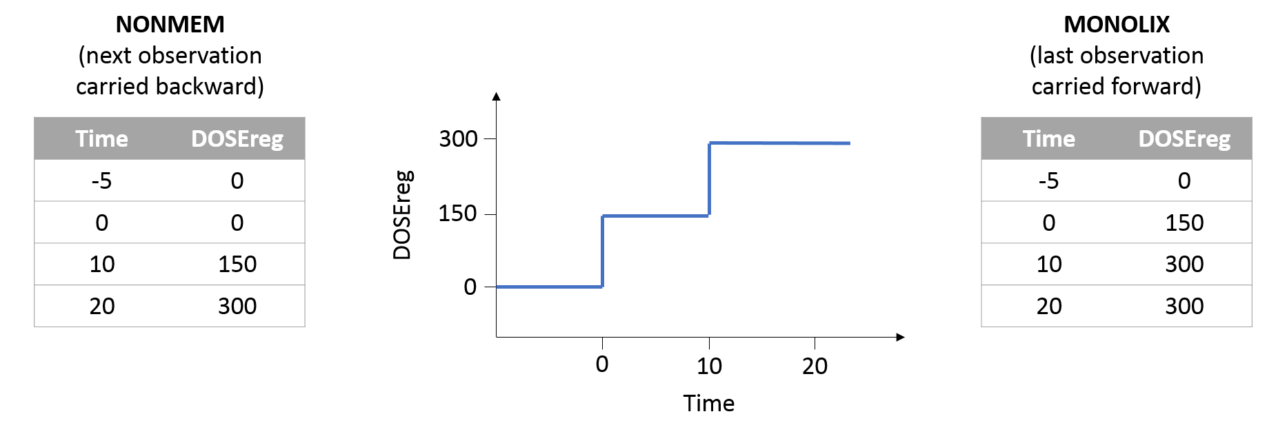
Unsupported column-types
- The PCMT, CONT, CALL, MRG_, RAW_, RPT_, L1, and L2 column-types are not supported in the MonolixSuite.