- OBSERVATION (formerly Y): response
- OBSERVATION ID (formerly YTYPE): response identifier
- CENSORING (formerly CENS): censored observation
- LIMIT: limit for censored values
OBSERVATION (formerly Y): response
The OBSERVATION column-type can be used to record continuous, categorical, count or time-to-event data. For dose lines, the content is free and will not be used. For response lines, the requirements depend on the type of data and are summarized below. Note that the interpretation of dose and response lines has changed between the 2016R1 and the 2018R1 versions, as detailed here.
For continuous data:
The value represents what has been measured (e.g concentrations) and can be any double value.
Examples:
- Basic example:
ID TIME AMT   Y
1   0   50     .
1 0.5    .   1.1
1   1    .   9.2
1 1.5    .   8.5
1   2    .   6.3
1 2.5    .   5.5
- Full data set for continuous data: theophylline data set, the warfarin data set, and the HIV data set
For categorical data:
In case of categorical data, the observations at each time point can only take values in a fixed and finite set of nominal categories. In the data set, the output categories must be coded as consecutive integers.
Examples:
- Basic example:
ID TIME Y
1 0.5   3
1   1   0
1 1.5   2
1   2   2
1 2.5   3
- Full data set for joint continuous and categorical data: warfarin data set.
For count data:
Count data can take only non-negative integer values that come from counting something, e.g., the number of trials required for completing a given task. The task can for instance be repeated several times and the individuals performance followed.
Count data can also represent the number of events happening in regularly spaced intervals, e.g the number of seizures every week. If the time intervals are not regular, the data may be considered as repeated time-to-event interval censored, or the interval length can be given as regressor to be used to define the probability distribution in the model.
Examples:
- Basic example: in the data set below, 10 trials are necessary the first day (t=0), 6 the second day (t=24), etc.
ID TIME  Y
1   0   10
1  24    6
1  48    5
1  72    2
For (repeated) time-to-event data:
In this case, the observations are the “times at which events occur“. An event may be one-off (e.g., death) or repeated (e.g., epileptic seizures, mechanical incidents, strikes). In addition, an event can be exactly observed, interval censored or right censored.
For the formatting of time-to-event data, the column TIME should contain not only the time of an event, but also other relevant times such as the start and end of the observation period or time intervals for interval-censoring. The column OBSERVATION contains an integer that indicates how to interpret the associated time. The different values for each type of event and observation are summarized in the table below:
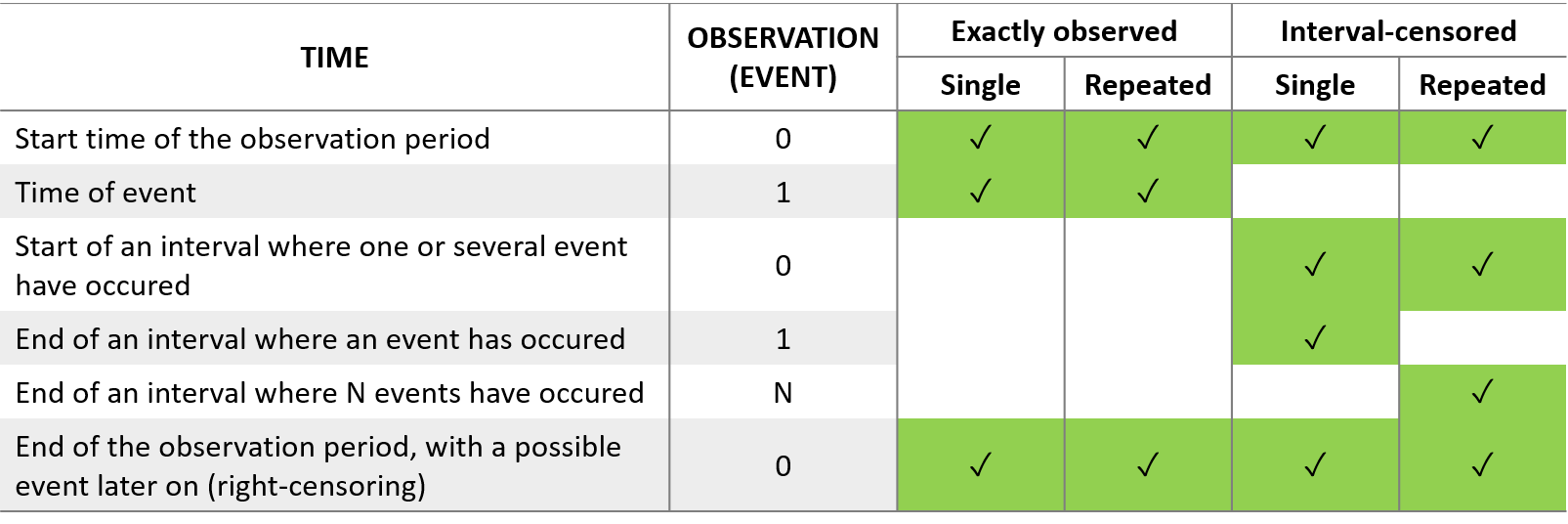
The figure below summarizes the different situations with examples: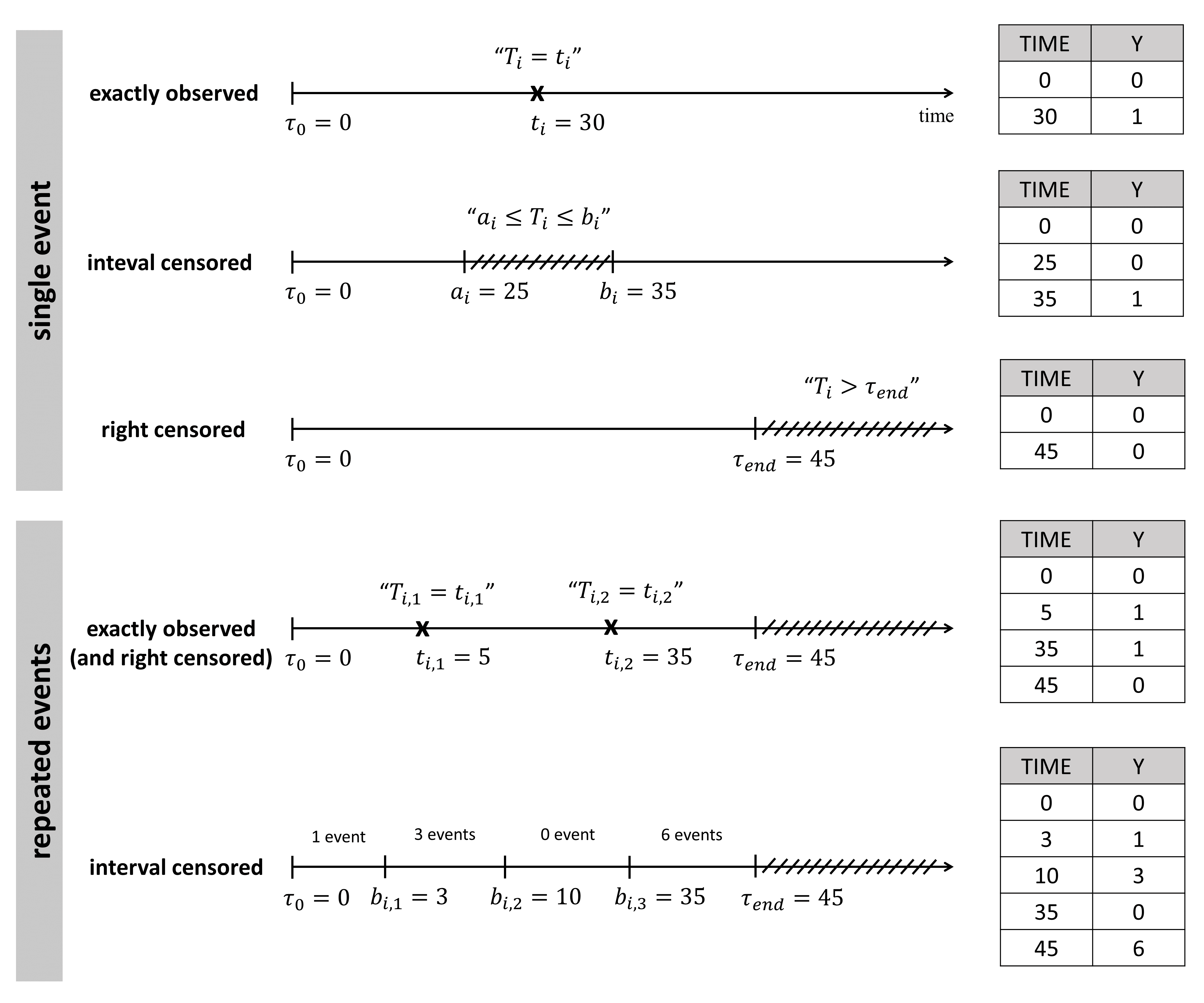
For single events exactly observed:
One must indicated the start time of the observation period with Y=0, and the time of event (Y=1) or the time of the end of the observation period if no event has occurred (Y=0).
Examples:
- Basic example: in the following dataset, the observation period last from starting time t=0 to the final time t=80. For individual 1, the event is observed at t=34, and for individual 2, no event is observed during the period. Thus it is noticed that at the final time (t=80), no event occurred.
ID TIME Y
1   0   0
1  34   1
2   0   0
2  80   0
- Full data sets for time-to-event data: PBC data set and Oropharynx data set
For repeated events exactly observed:
One must indicate the start time of the observation period (Y=0), the end time (Y=0) and the time of each event (Y=1).
Examples:
- Basic example: below the observation period last from starting time t=0 to the final time t=80. For individual 1, two events are observed at t=34 and t=76, and for individual 2, no event is observed during the period.
ID TIME Y
1   0   0
1  34   1
1  76   1
1  80   0
2   0   0
2  80   0
For single events interval censored:
When the exact time of the event is not known, but only an interval can be given, the start time of this interval is given with Y=0, and the end time with Y=1. As before, the start time of the observation period must be given with Y=0.
Examples:
- Basic example: we only know that the event has happened between t=32 and t=35.
ID TIME Y
1   0   0
1  32   0
1  35   1
For repeated events interval censored:
In this case, we do not know the exact event times, but only the number of events that occurred for each individual in each interval of time. The column-type Y can now take integer values greater than 1, if several events occurred during an interval.
Examples:
- Basic example: No event occurred between t=0 and t=32, 1 event occurred between t=32 and t=35, 1 between t=35 and t=50, none between t=50 and t=56, 2 between t=56 and t=78 and finally 1 between t=78 and t=80.
ID TIME Y
1   0   0
1  32   0
1  35   1
1  50   1
1  56   0
1  78   2
1  80   1
Format restrictions
- A data set shall not contain more than one column with column-type OBSERVATION.
- If EVENT ID = 1, 3 or 4, the content of the OBSERVATION column is free and ignored.
- If EVENT ID = 0, and IGNORED OBSERVATION = 1 or 2, the content of the OBSERVATION column is free and ignored.
- If EVENT ID = 0 and IGNORED OBSERVATION = 0, the contant of the OBSERVATION column has to be a double (dots ‘.’ are not allowed).
- If the EVENT ID column is absent (and whatever the IGNORED OBSERVATION column is), the content is free. Values that are not doubles (for instance dots ‘.’ or strings) are ignored.
Warnings
- If a subject or a subject-occasion has no observations, a warning message arises telling which subjects or subjects-occasions have no measurements and will be ignored.
FAQ
- My data is not “over time”, what should I do? You can arbitrarily set the time of each observation to 0.
OBSERVATION ID (formerly YTYPE): response identifier
The OBSERVATION ID column permits to distinguish several types of observations (several concentrations, effects, etc). The OBSERVATION ID column assigns an identifier to each observation of the OBSERVATION column. Those identifiers are used to map the observations of the data set to the outputs of the model (in the OUTPUT block of the Mlxtran model file). The mapping is done following alphabetical order: the first OBSERVATION ID value in alphabetical order is mapped to the first output in the output list, etc. We recommend to use integers (1, 2, …) as identifiers, such that the observations with identifier 1 are mapped to the first output, observations with identifier 2 to the second, etc. If you have more than 10 different outputs, note that in alphabetical order ’10’ become ‘2’. In that case using letters (a, b, c, …) as identifiers is more intuitive. The dot “.” is not considered as a repetition of the previous line but as a different identifier.
There can be more OBSERVATION ID values than there are outputs in the model file. In that case only the observations corresponding to the first identifiers(s) in alphabetical order will be used (example below).
For continuous data, in the Monolix graphical user interface, the data viewer and the plots, the observations will be called yX with X corresponding to the identifier given in the OBSERVATION ID column (for instance y1 and y2 if identifiers 1 and 2 were used in the OBSERVATION ID column).
Examples:
- Basic example with integers: with the following data set
TIME AMT OBS YTYPE
 0   .   12   1
 5   .    6   2
10   .    4   1
15   .    3   2
and the following output block
OUTPUT:
output = {Cc, R}
the observations “12” and “4” which have identifier “1” will be matched to the output “Cc”, while observations ”6″ and “3” with identifier “2” will be matched to “R”.
- Basic example with strings (not recommended): with the following data set
TIME AMT OBS YTYPE
 0   .   12  PK
 5   .    6  PK
10   .    4  PD
15   .    3  PD
and the following OUTPUT block in the Mlxtran model file:
OUTPUT:
output = {Cc, R}
the observations tagged with “PD” will be mapped to the first output “Cc” (which is probably not what is desired), and those tagged with “PK” will be mapped to the second output “R”, because in alphabetical order “PD” comes before “PK”.
- Basic example with more OBSERVATION ID values than model outputs: with the following data set
TIME AMT OBS YTYPE
 0   .   12   1
 5   .    6   2
10   .    4   1
15   .    3   2
and the following output block
OUTPUT:
output = {Cc}
the observations tagged with identifier “1” will be mapped to the model output “Cc” and the observations tagged with “2” will be ignored. If the user wants to use only the data tagged with “2”, he can add an IGNORED OBSERVATION column which ignores all observations with identifier “1” (see below).
- Basic example with more OBSERVATION ID values than model outputs and an IGNORED OBSERVATION column: with the following data set
TIME AMT OBS YTYPE MDV
 0   .   12   1     1
 5   .    6   2     0
10   .    4   1     1
15   .    3   2     0
and the following output block
OUTPUT:
output = {Cc}
the observations tagged with identifier “1” will all be ignored (due to the MDV column tagged as IGNORED OBSERVATION) and the observations with identifier “2” will be mapped to the model output “Cc”.
- Full data set example: warfarin PKPD data set, PSA and survival data set
Format restrictions:
- A data set shall not contain more than one column with column-type OBSERVATION ID.
- The content of the OBSERVATION ID column can be strings or integers.
- The dot “.” is not considered as a repetition of the previous line but as a different identifier.
CENSORING (formerly CENS): censored observation
The CENSORING column permits to mark censored data. When an observation is marked as censored, the (upper or lower) limit of quantification is given in the OBSERVATION column (not in a separate column).
- CENSORING = 1 means that the value in OBSERVATION column (that we call \(y_{obs}\) here) is an upper limit. The true observation y verifies \(y<y_{obs}\).
- CENSORING = 0 means the value in response-column corresponds to a valid observation (no interval associated).
- CENSORING = -1 means that the value in OBSERVATION column (\(y_{obs}\)) is a lower bound. The true observation y verifies \(y>y_{obs}\).
The mathematical handling of censored data is described here.
Format restrictions:
- A data set shall not contain more than one column with column-type CENSORING.
- For dose lines, the content is free and will be ignored.
- For response lines, there are only four possible values : -1, 0, 1 and ‘.’ (interpreted as 0).
LIMIT: limit for censored values
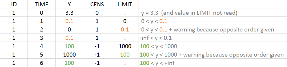
When the column LIMIT contains a numeric value and CENSORING is different from 0, the value in the LIMIT column is interpreted as the second bound of the interval. Writing \(y_{obs}\) the value in the OBSERVATION column and \(y_{limit}\) the value in the LIMIT column, the true observation y verifies \(y\in [y_{limit}, y_{obs}]\). When LIMIT = ‘.’ , the value is interpreted as -infinity or +infinity depending on the value of CENSORING (1 or -1 respectively) as if the LIMIT column would not be present.
Format restrictions:
- A data set shall not contain more than one column with column-type LIMIT.
- A data set shall not contain any column with column-type LIMIT if no column with column-type CENSORING is present.
- Allowed values are doubles and dot ‘.’ , and strings are not allowed (even when CENSORING = 0).
Example with CENSORING and LIMIT
It is possible to have both censoring type on the same individual, i.e. both upper or lower limit of quantification. It is possible to have measurements with and without bounds. The example below gives an overview of the possible combinations: